SO441 Synoptic Meteorology

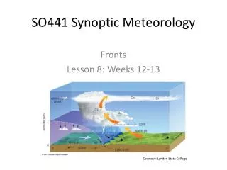
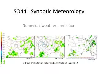
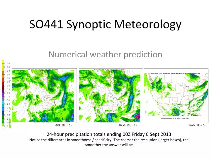
1. SO441 Synoptic Meteorology Numerical weather prediction GFS: 23km Δx NAM: 12km Δx NAM: 4km Δx 24-hour precipitation totals ending 00Z Friday 6 Sept 2013 Notice the differences in smoothness / specificity! The coarser the resolution (larger boxes), the smoother the answer will be

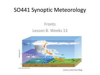
2. A bit of important history . . . • What is numerical weather prediction? • An integration forward in time (and space) of fundamental governing equations: 6 equations, 6 unknowns • Equation of state • Navier Stokes (from F=ma) • Continuity equation • Thermodynamic energy equation (from 1st & 2nd laws of thermodynamics) • Why is it so important? • Moved meteorology away from a collection of rules-of-thumb and educated guesses to an analytic science grounded in physics and calculus

3. What, exactly, is a dynamical model? • A set of computer programs/lines of code (usually written in FORTRAN), designed to simulate the real atmosphere • Integrate the primitive equations forward in time to solve them at each grid point • Use “finite differencing” techniques to evaluate partial derivatives • What does a dynamical model need to succeed? • A good set of governing equations • Accurate initial and boundary conditions • Remember Dr. Lorenz’s experiment with rounding? • What is “success”? • Large grid boxes – give “smoother” answers than smaller grid boxes • In 2013, global models have grid boxes around 25 km, while regional models are between 5 and 10 km

4. Finite differencing: a simple example • Using data from the Oklahoma Mesonet (right), can we calculate the temperature advection in Tulsa, OK (very close to the home of SOC 2/C Justin Engel) at 2100 UTC 04 Sept 2013? • Then, based on our calculation, can we quantitatively predict the temperature in Tulsa at 2200 UTC 04 Sept 2013 (holding all else constant)? (adapted from Lackmann 10.2, pg. 250)

5. Finite differencing: a simple example • To setup the model, even though this is a simple example, we actually still need to make 4 assumptions about the factors influencing temperature in OKC • Temperature advection (transport of air to a new location) is the dominant factor • Diurnal heating or cooling is not important • Processes relating to clouds and precipitation do not come into play • If these assumptions are made, the governing equation for temperature uses the following: • Which says: “Quantity changes in time at a fixed point because of advection at that point”. • Temperature advection then becomes: • Where u is the east-west wind, v is the north-south wind, and x and y are the distances in east-west and north-south directions, respectively. (Note: vertical advection, with wand z, is conveniently ignored here)

6. Finite differencing: a simple example • Tulsa is located at the point (i,j), and we know the temperature at the point (i-1,j+1) and (i,j). We also know the wind is now blowing from the ENE (out of 20°) at 5 knots. Let’s discretize the advection equation:

7. Finite differencing: a simple example • Rearrange the advection equation to solve for the final temperature: • Plugging in the numerical values from the figure, we see that the predicted temperature at 2200 UTC will be about 0.1°F warmer than the temperature at 2100 UTC, all because of advection!

8. Grid spacing in a model From: http://www.drjack.info/INFO/model_basics.html In the upper-left figure, the point represent the centers of hypothetical grid boxes. Most models stagger their solutions, solving the wind (u,v,w) at the edges of the boxes and the mass (temp, mixing ratio, height/pressure) at the centers

9. Parameterizations • For all processes that take place inside a grid box, i.e., they are smaller than the grid spacing of the model, the model cannot “resolve” them explicitly • Processes requiring parameterization: • Planetary boundary layer • Turbulence (energysmaller scales) • Flux of momentum, heat, and water vapor • Land-surface • Water and water vapor cycle • Microphysics (clouds) • Precipitation The effects that model physics parameterizations attempt to simulate are generally unresolvable at grid scales

10. Parameterizations: planetary boundary layer • Turbulent fluxes need to be “transported” from within the planetary boundary layer to outside it • Example: momentum flux in the governing equation for u: • Similar equations exist for other flux quantities: • Heat • Water vapor Example of the “boundary layer”

11. Parameterizations:Land-surface models • Many complex processes to “pass” on to the model: • Evaporation • Transpiration • Infiltration/runoff • Sublimation • Condensation • Note that nearly all have something to do with water!

12. Parameterizations:Cloud microphysics • Imagine a cloud occupies a model 3-d grid box • How many water molecules are there? • What shapes/sizes are those molecules? • What phases of water (gas, liquid, solid) are present? • Is there more condensation/freezing • And thus heat being added to the atmosphere • Or is there more evaporation/melting • And thus heat being removed?

13. Parameterizations:Cumulus parameterization • Clouds come in many shapes and sizes • Most clouds are between 0.5-3 km in diameter • Thus smaller than model grid boxes • To get precipitation in the model, need to parameterize clouds • “Trigger” precipitation when certain thresholds are met: relative humidity above 70-80%, positive w (rising motion), CAPE • Effect is to warm and dry the atmosphere above the surface • Multiple “schemes” for cumulus parameterization: each differs in how it adjusts the atmosphere column in response to precipitation • Betts-Miller-Janic • Arakawa-Schubert • Kain-Fritsch

14. Parameterizations:Cumulus parameterization • Example: how to handle precipitation in a model grid cell • Difference between cloud water for an explicit (a) vs. parameterized (b) precipitation event

15. Data assimilation • What is data assimilation? • A means of combining all available information to construct the best possible estimate of the state of the atmosphere • What data are assimilated? • In-situ surface observations: temp, dew point, pressure, cloud cover, wind speed and direction, current weather, visibility • Like the weather station we have on the field out at the corner of Hospital Point • Ships, buoys • In-situ upper-air observations • Radiosondes, aircraft • Remotely sensed observations • Satellites: clouds, but also temperature, water vapor, and even vertical profiles • Radar: precipitation, air motion • GPS radio occultation Radiosonde network ACARS observations

16. Data assimilation • How does it work? • Observations must be blended together and interpolated to the nearest model grid point (horizontal and vertical) • Not an easy process! • Which data source is most important? • Sensitivity studies (data denial) show that it depends Flow chart for the GFS model Data sources: Radiosondes, ACAR, and surface Sensitivity of the u-wind forecast to the various components

17. Ensemble modeling • Predicting future weather using a suite of several individual forecasts • Idea began with Ed Lorenz at MIT in 1950s: tried to repeat an experiment he had made with an equation. Found that very small rounding differences completely changed the mathematical answer! • This is now known as the “butterfly effect”: an even miniscule difference in the initial state will eventually amplify and result in a different forecast • Lorenz proposed an upper-limit on weather forecasts of 2 weeks • Also found that some situations “degrade” much faster than others • Ensemble weather prediction attempts to show how fast the solutions “degrade”

18. Why are there still errors in NWP today? • Grid spacing • The atmosphere is divided into cells, and the center point (or edge points) is (are) forecasted • Topography, ground cover, etc. vary – sometimes dramatically – inside one grid box (but the forecast for that grid box gives only one unique value) • Equations of motion are non-linear • Changes in one variable feed back to all others • Differential equations are solved by discretizing them in time • Rounding occurs in finite-differencing techniques • This noise, as found by Dr. Lorenz, leads to growing error • Initial conditions • Current atmospheric state is unknown at all points • Parameterizations • Sub-grid processes are estimated