Download
1 / 17
170 likes | 279 Views
Surplus Measures. An Alternative View of the Demand Curve. An alternative interpretation of the demand curve is that it represents the consumer’s marginal willingness to pay or $marginal benefit for the quantity specified.

E N D
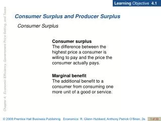
An Alternative View of the Demand Curve • An alternative interpretation of the demand curve is that it represents the consumer’s marginal willingness to pay or $marginal benefit for the quantity specified. • So, another way of looking at the demand curve is that it tells you the $marginal benefit at each unit of consumption. • $Total benefit of consumption would then be the sum of all the marginal benefits up to, say, X units.
Willingness to Pay • Think of the total amount you would pay for X units (say it is $27) and then for X-1 units (say it is $25). Your marginal willingness to pay for that Xth unit is $2 (= 27 -25). • Alternatively, we could say that your quantity demanded at the price $2/unit is X because you are willing to pay up to $2/unit for the Xth unit.
Consumers Surplus • For one individual: consumer’s surplus (CS) is the difference between the consumer’s total willingness to pay ($total benefit) and what the consumer actually did pay ($total expenditure). • CS = the area between the consumer’s demand curve and the market price line. • To go from individual consumer’s surplus to market consumers’ surplus, just use the market demand, which aggregates all the individuals.
Example: Li’s Willingness to Pay for Wheat and Consumer Surplus • The table at the right shows Li’s willingness to pay for the indicated quantities of wheat. • Her marginal marginal willingness to pay (marginal benefit) is the difference between her willingness to pay for X and X-1 units of wheat. • Li’s demand curve would be the plot of her marginal willingness to pay against number of units. • Marginal consumer surplus on each unit is the difference between marginal willingness to pay and the price she actually pays, PW=$2/lb in this example. • Total consumer surplus is the sum of all entries in the marginal consumer surplus column.
Consumer Surplus and Quantity Demanded • If the price of wheat is $2/lb., then Li buys 10 lbs. of wheat, the point where her marginal benefit of wheat equals its price. • Notice that the marginal willingness to pay column (marginal benefit) is just Li’s demand for wheat. • When PW=$2 and W=10, Li’s consumer surplus is $72.50, indicating that she would have been willing to pay an additional$72.50 for the wheat she consumed (above the $20 she had to pay). • Try it for PW = $4.00
Graphical Measure of Li’s Consumer Surplus • The area under the demand curve and above the market price is the total consumer surplus. • The arrow on the right shows Li’s total consumer surplus when the market price of wheat is $2/lb.
Market Consumer Surplus Question • The table at the right is a sample market demand curve. • Question: At a market price of $2.00, what is the total consumer surplus?
Market Consumer Surplus Answer • At a market price of $2.00, total expenditures are $14 = 7 x $2.00 • Total willingness to pay is $40 = 12 + 8 + 6 + 5 + 4 + 3 + 2. • Total consumer surplus = $40 - $14 = $26. • Total consumer surplus = sum of marginal consumer surplus = 26 = 10 + 6 + 4 + 3 + 2 + 1 + 0.
Graph of Market Consumer Surplus • As in the case of individual consumer surplus, the area below the demand curve and above the market price measures the total market consumer surplus.
Why Measure Consumer Surplus? • An individual’s total consumer surplus on a purchase measures the gain to the consumer from the market transaction. • In the market as a whole, the total consumer surplus measures the gain to society from the existence of the market equilibrium price.
Producers Surplus • Producers surplus measures the gain to firms from selling all units at the market price. • Producers surplus is the supply-side equivalent of consumers surplus. • Think of the supply curve as measuring the marginal costs of production. • For one firm: producer’s surplus (PS) is the difference between what the firm gets in revenue ($total revenue) and what the sum of the marginal costs are ($total variable costs). • PS = the area between the market price line and the firm’s supply curve. • To go from individual producer’s surplus to market producers’ surplus, just use the market supply, which aggregates all the firms.
Producers Surplus • Suppose the market equilibrium occurs at P* & X*. • Total revenue to producers is the area OP*BX*. • Sum of marginal costs is the area OABX*. • Producers surplus is the red shaded area AP*B. P Supply=MC P* B Demand=MB A Quantity X* O
Demand and Supply Revisited • Market demand reflects marginal benefit. • Market supply reflects marginal costs. • Consumers surplus measures the gains from trade to the consumers. • Producers surplus measures the gains from trade to the producers. • Total gains from trade - or total surplus - or net social surplus - is the sum of consumers and producers surplus. It can also be thought of as $total benefit-sum of $marginal costs.
Net Social Surplus • The market equilibrium occurs at P* & X*. • $TB = area OCBX* • $total expenditure = area OP*BX* • $CS is the top blue shaded area P*CB • $total revenue =area OP*BX* • sum of $mc = OABX* • $PS = bottom red shaded area AP*B • $Net social surplus = area ACB = the top and bottom triangles. $ Supply=MC C B P* Demand=MB A Quantity X* O
Selling My House • Old address: 133 Tompkins St. • New address: 132 Tompkins St. • Problem: we bought the new house before selling the old one. • Our minimum selling price (after 2 years) = $55,000. • Potential buyer Abe: maximum buying price = $45,000 • So, no deal with Abe.
Selling My House • Potential (and last) buyer Betty: maximum price = $95,000 • Trade should occur! Net social surplus on trade = $40,000 • Remember: Our minimum selling price (after 2 years) = $55,000. • Division of surplus to the Wissink’s and to Betty depends on the strike price - what we sell the house for. • Suppose we sold it for $90,000. • HA! • Consumers surplus=$5,000 and Producers surplus=$35,000. • What did we sell it for? • Don’t ask!