Download
1 / 59
590 likes | 594 Views
3. Advanced Routing Protocols and IPv6. 3.1 Traditional IP Routing 3.2 Multicast IP 3.3 CacheCast 3.4 AODV for Mobile AdHoc Wireless LANs (MANETs) 3.5 IPv4 and IPv6. Traditional IP Routing.

E N D
3. Advanced Routing Protocolsand IPv6 • 3.1 Traditional IP Routing • 3.2 Multicast IP • 3.3 CacheCast • 3.4 AODV for Mobile AdHoc Wireless LANs (MANETs) • 3.5 IPv4 and IPv6
Traditional IP Routing • IP is a datagram protocol, i.e., every packet is routed separately, indepen-dent of earlier packets. Every packet contains the full IP address of the re-ceiver (and the sender). Traditional IP was designed for wired networks. It uses a distributed routing strategy, i.e., the routes are decided jointly by different nodes. The nodes exchange information to come up with good routes and to deal with chan-ging network conditions.
Distance Vector Routing (1) • Principle • The nodes explicitly exchange routing information with their neighbors: • Each node knows his own distance to every neighbor: • number of hops (= 1) • delay (round-trip time) • queue length (indication for congestion) • etc. • Each node periodically sends a list E with his estimated distances to all known destination nodes to his neighbors. • Node X receives such a list E from neighbor Y • distance (X, Y) = e • distance (Y, Z) = E(Z) • => distance (X, Z) over Y is E(Z) + e • The table with these distances is called distance vector. The algorithm is thus called distance vector routing.
A B C D E F G H J K L I Distance Vector Routing (2) • Example We consider the delays known to node J. Note that delays are not necessarily symmetric.
Distance Vector Routing (3) Right column: newly determined delays at node Jafter receiving the distance vectors from the neighbors.
RIP • In theearlyyearsofthe Internet themostwidelyusedinteriorrouting proto-col (withinAutonomous Systems) was distancevectorrouting. The emplo-yedprotocol was calledRIP (Routing Information Protocol). • With RIP all internetroutersperiodicallyexchangedistancevectormes-sagesand update theirroutingtablesaccordingly.
B C From B From C link cost link cost to to A bc 2 A ab 1 bc ce B bc 1 E C bc 1 D cd 1 D bc 2 From E link cost E ce 1 ab to cd C ce 1 D A D de 1 From D de From A link cost link cost to to ad A ad 1 B ab 1 B cd 2 C ab 2 C cd 1 D ad 1 E de 1 Another Example for Distance Vector Routing (1) • (a) node E has just been added to the network
B C From B From C link cost link cost to to A ab 1 A bc 2 bc ce C bc 1 B bc 1 E D bc 2 D cd 1 From E link cost E bc 2 E ce 1 ab to A de 2 cd D A B ce 2 C ce 1 From D From A de link cost link cost D de 1 to to ad A ad 1 B ab 1 B cd 2 C ab 2 C cd 1 D ad 1 E de 1 E ad 2 Example for Distance Vector Routing (2) (b) after an exchange of RIP messages
Hierarchical Routing • The sizeoftheroutingtablesis proportional tothesizeofthenetwork: • large memoryrequirement in thenodes • considerable CPU time forsearchingthetables • muchbandwidthfortheexchangeofroutinginformation • Hierarchicalroutinghelpstosolvetheseproblems: • Nodes aregroupedintoregions • Eachnodeknows • all detailsofhisregion • hisroutesto all otherregions • In the Internet a “region” is a subsetofthe IP addressspace. • Disadvantage:globally optimal decisionsarenolongerfound.
full table for node 1A hierarchical table for node 1A DES. LINE HOP LINE HOP DES. 1A - - 1A - - region 1 1B region 2 2A 2B 1B 1B 1 1B 1B 1 1C 1C 1 1C 1C 1 2A 1B 2 2 1B 2 2C 2D 1A 1C 2B 1B 3 3 1C 2 2C 1B 3 4 1C 3 2D 1B 4 5 1C 4 4B 5B 5C 3A 1C 3 3A 3B 3B 1C 2 5A 5D 4A 1C 3 5E 4A 4C 4B 1C 4 region 3 region 4 region 5 4C 1C 4 5A 1C 4 5B 1C 5 5C 1B 5 5D 1C 6 5E 1C 5 Example for Hierarchical Routing
OSPF Routing (1) • The mostwidelyusedinteriorroutingprotocol in the Internet todayisOSPF (Open Shortest Path First). The basicideaisthat all nodesknowtheentirenetworktopologyat all timesandcanthuscompute all optimal pathslocally. • Ifthetopologychanges, thenodesexchangetopology update messages. Eachnodemaintains a local “database“ oftheentiretopology, calledthelink statedatabase. • The optimal pathsto all destinationscanbecomputedlocallywithDijkstra‘sShortest Path algorithm (Shortest Path First = SPF). In the Internet slangthealgorithmisthuscalled “Open Shortest Path First“. • Algorithmsofthisclassare also called ”link stateroutingalgorithms”.
OSPF Routing (2) • Requirements when RIP was replaced by OSPF • The new protocol had to support a variety of distance metrics, including physical distance, delay, and so on. It had to be a dynamic algorithm, one that adapted to changes in the topology automatically and quickly. • The new protocol had to do load balancing, splitting the load over multiple lines. Most previous protocols sent all packets over the best route, the second-best route was not used at all. In many cases, splitting the load over multiple lines gives better performance. • Support for hierarchical systems was needed. By 1988, the Internet had grown so large that no router could be expected to know the entire topology. The new routing protocol had to consider routes to subnetworks as desti-nations.
bc ab cd de ad Example for OSPF Routing • (a) network in stable condition B C ce E D A (b) links bc and ad failed (c) after an exchange of OSPF messages
3.2 Multicast IP Definition of Multicast The transmission of a data stream from one sender to multiple (but not all) receivers is called multicast. Multicast is especially important for multimedia data streams: • Multimedia applications often require 1:n communication. Examples: • Video conferences • Tele-cooperation (CSCW) with a shared work space • Near-Video-on-Demand • Broadcast of radio and TV • Digital video streams have very high data rates. A transmission over n point-to-point connections can easily cause an overload of the network.
S S n end-to-end connections one multicast connection Motivation for Multicast • More „intelligence" in the inner nodes of the network reduces • the load of the sender • the load on the links
Multicast in LANs • Ethernet, Wireless LAN, etc. • The topology has broadcast characteristics. • The layer-2 addresses according to IEEE 802 allow the use of group addresses for multicast. Thus, multicast can easily and efficiently be realized in a LAN segment. • But: For a long time, in layer 3 and higher layers of the Internet protocol architecture, only peer-to-peer (unicast) addresses were supported!
Multicast in the Network Layer • Principle: Duplication of packets as "deep down" in the multicast tree as possible. Multicast in WANs requires • a multicast address mechanism in layer 3 and more "intelligence" in layer 3 routers. • extensions to the routing tables • new routing algorithms
bc B C c e b a cd E e d ad A D Example Topology
B B C C E E A A D D The Advantage of Multicast in the Example Topology • (b) one multicast connection (a) four unicast connections
Routing Algorithms for Multicast • Multicast routing has been realized for the Internet in layer 3 (multicast IP). • The employed routing algorithms are extensions of the unicast routing algo-rithms; they are compatible with these. • Multicast in the Internet is receiver-oriented. For a multicast session all participants (sender and receivers) agree on a multicast address. The sen-derbegins to send to this address. Each node in the Internet can then de-cidewhether it would like to be included into an existing multicast session and receive the data traffic.
Principles of Multicast IP • IP packets are transmitted to a group address (IP address of type D). • connectionless service (datagram service) • best-effort principle (no quality of service guarantees): • no error control • no flow control • no guarantee that the packet order is maintained. • receiver-oriented: • The sender sends multicast packets to the group. • The sender does not know the receivers, has no control of them. • Each host on the Internet can join a group. • A restriction of the transmission range is only possible by the Time-To-Live parameter (TTL = hop counter in the header of the IP packet).
Multicast Addresses in IP • The IP groupaddress was standardizedas IP addressofclass D. Ithasnonetid/hostidstructure, itimplements just a flat numberspace. • Group addressesareassigneddynamically. Thereisnomechanismfortheuniqueassignmentof a groupaddress in IP! Higher layershavetotakecareofaddressassignmenttogroups.
Third round Second round First round Routing Algorithms for Multicast • Flooding • The simplestpossibilityforreaching all receiversof a groupwouldbeflooding (broadcasting). • AlgorithmFlooding • When a packet arrivesat a node, a copyissenttoeachoutgoing link excepttheone on whichitcame.
Reverse Path Broadcasting (RPB) • More efficientthanfloodingistheReverse Path Broadcastingalgorithm (RPB). Itusesthefactthateachnodeknowsitsshortestpathtothesenderfromtheclassical (point-to-point) routingtable! ThispathiscalledtheRe-verse Path. • The firstideaisnowthat a nodeforwardsonlythosepacketstohisneigh-borsthathavearrived on theshortestpathfromthesender. • Thisalgorithmgeneratessubstantiallyfewerpacketsthanflooding.
Example of Reverse Path Broadcasting (incomplete algorithm) • For our example topology the (so far still incomplete) RPB algorithm works as follows: B C bc ce E ab cd A de D ad As we see, there are still redundant packets: nodes D and E receive every packet twice, node C even three times.
Reverse Path Broadcasting (complete algorithm) • If each node communicates additional information to his neighbors, RPB can prevent all redundant packets. The additional information consists of the fact whether the neighbor is on his shortest path to the sender. • In our example, E informs his neighbors C and D that D lies on his shortest path to A. A node will then forward packets only to those "sons" from whom he knows that he lies on their shortest path to the sender. The diagram be-low shows the packet flow for the full RPB algorithm. B C bc ce E ab cd A de D ad
Truncated Reverse Path Broadcasting (TRPB) • TRPB limits the distribution of the data to those subnetworks that contain multicast group members. Only LANs that are leaves of the routing tree are considered. • A simple group management protocol was defined for this purpose: the rou-ter asks the hosts in his LAN whether they are interested in receiving the packets of a certain group. They reply with yes or no. If a router has no inter-ested host in his LAN, he will no longer forward packets with this group ad-dress into his LAN (IGMP: Internet Group Management Protocol). • Advantage • Avoids unneccessary traffic in the leaf LANs. • Disadvantage • Can eliminate only leaf subnetworks, does not reduce the data traffic at the higher levels of the tree.
Reverse Path Multicasting (RPM) • It obviously makes sense to cut back the routing tree in the data phase of a multicast session so that packets are only forwarded to those subtrees where there are interested receivers. • This is done with so-called "prune messages". They propagate from the leaves towards the root of the tree and communicate to the upstream nodes that there are no interested receivers further down in the tree. In this way a broadcast tree becomes a multicast tree. The algorithm is called Reverse Path Multicasting (RPM). • In the Internet the protocol that implements the RPM algorithm is called DVMRP(Distance Vector Multicast Routing Protocol).
Algorithm “Pruning” • A router whose sons are not interested in the multicast session sends a Non-Membership Report (NMR) to the upstream router, i.e., to the higher-level router in the multicast tree. • A router who received NMRs from all his downstream routers send a NMR to his upstream neighbor. • NMRs come with a timeout after which the pruning is canceled. This allows new, joining hosts at lower levels of the tree to find out about all ongoing multicast sessions. • NMRs can also be canceled by an explicit message (the craft message) if a host below a link becomes interested in the session again.
Example for Reverse Path Multicasting • (a) tree in the initial RPB phase (c) D has sent a "prune message" (b) E has sent "prune message" B C bc ce E ab cd A de D ad
Advantages and Disadvantages of RPM • Advantage • Reduction of data traffic compared to TRPB • Disadvantages • Periodic flooding of the data to all routers is necessary so that they can reconsider their decision. • Status information for each group and for each sender must be main-tained in each node. • For each pair (sender, group address) a separate routing tree must be created.
Core-Based Trees • All algorithms represented so far have the disadvantage that for every (sen-der, group) pair a separate multicast tree must be created and maintained. Core based trees avoid this disadvantage. Only one tree per group is built. Every sender sends to the same tree. • Today‘s most advanced multicast routing protocol in the Internet is called PIM-SM (Protocol Independent Multicast - Sparse Mode). It is based on the idea of core-based trees.
3.3 CacheCast • Failure of IP Multicast • More than two decades of research resulted in so called multicast isles. • Only 2.2% of total ASes are multicast enabled, and the percentage is decreasing. • What’s wrong with IP Multicast? • There are technicaland commercialissues I would like to thank Dr.PiotrSrebrny and Professor Thomas Plagemann for their help with the transparencies onCacheCast. This work was done at the University of Oslo, Norway.
Technical Issues • Scalability wrt. memory and CPU processing • IP multicast requires per-flow state • Security • Lack of protection against attacks on routers and sessions • Congestion control • Group management • sender/receiver authorization, group management not well defined • No support for mobile devices
Commercial Issues • Payment model violated • Who pays? The number of downstream receivers is unknown. • Not explicitly incrementally deployable
CacheCast • CacheCast is a link-level caching mechanism that eliminates redundant data trans-missions. • Caching is a very useful technique to improve performance.
CacheCastIdea (1) • A packet with a payload P is destined to A • It traverses a set of routers leaving a copy of the payload P and marking the outgoing interface • Second packet with the same payload P is destined to B
CacheCastIdea (2) • The first router along the path discovers that the same payload P is on the next hop router and sends only the packet header. • The last router on the common path discovers that the payload P is not present on the next hop router in direction B and attaches it to the header.
Main Questions • How to determine the next hop cache contents? • How to construct the caches?
Cache Placement • Router = switching node • Packet behaviour highly indeterministic • Link = transmission channel • Packet behaviour is much more predictible
Link Cache • Caching is done per link: • Cache Management Unit (CMU) • Cache Store (CS) • The router remains untouched.
Link Cache Requirements • Very simple processing • ~72 ns to process a minimum size packet on a 10 Gb/s link and ~18 ns on a 40 Gb/s link • modern DDR read cycle ~20ns • modern SRAM read cycle ~5ns • Very small cache size: • The smaller the cache, the fewer items to match with the simpler processing • ~10 mscaches are sufficient (explained later)
Cacheable Packets • A CacheCastpacket carries metadata describing the packet payload: • Payload id • Payload offset • Index • Only packets with the metadata are cached!
Estimating Cache Size (1) • Concept of packet train • It is sufficient to hold payload P in the CS for time t. • To how many destinations can a source send a packet within time t?
Estimating Cache Size (2) • Back-of-the-envelope calculations
Implication of the Small Size • 10 mscache size on a 10 Gb/s link assuming 10 % of cacheable traffic: • ~1.28 MB for the CS storage space (fits SRAM memory) • ~1280 entries in the CMU table • What about a 100 Mb/s LAN? • ~13KB for CS • ~13 entries in the CMU table? • We can easily afford that!
Limited Cache Size • Assuming10ms caching time • A slow source is able to send only to few destinations within this time • If the caching time is exceeded the source must resend payload • This affects CacheCast efficiency