Download
1 / 25
250 likes | 264 Views
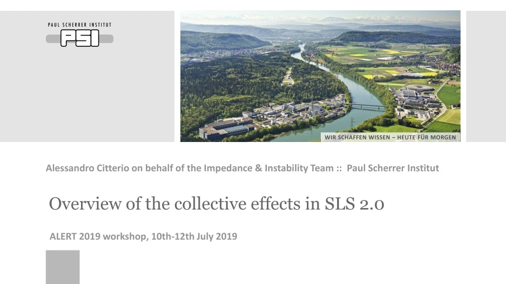
Alessandro Citterio on behalf of the Impedance & Instability Team :: Paul Scherrer Institut. Overview of the collective effects in SLS 2.0. ALERT 2019 workshop, 10th-12th July 2019. Contents. Co-authors: M.Aiba, M.Dehler, S.Dordevic, L.Stingelin.

E N D
Alessandro Citterio on behalf of the Impedance & Instability Team :: Paul Scherrer Institut Overview of the collective effects in SLS 2.0 ALERT 2019 workshop, 10th-12th July 2019
Contents Co-authors: M.Aiba, M.Dehler, S.Dordevic, L.Stingelin Overview of lattices (with negative momentum compaction) for the analysis of the collective effects (longitudinal & transverse) Microwave longitudinal instabilities: machine impedance for the SLS 2.0 lattice June '18 Longitudinal single bunch simulations without harmonic cavity • Longitudinal multibunch simulations with harmonic cavity • ELEGANT vs Mbtrack: code comparison • Landau Cavity, filling patterns • Threshold tendencies varyingparameter impedance • New lattices: impedance overview and threshold calculations Transverse single bunch effects (preliminary results) Characterization of NEG coatings SLS 1: validation of simulation model for the microwave instabilities Conclusions and outlook
upgrade projects transfer lines SLS: 17 years of very successful operation... ...but emittance 5 nm at 2.4 GeV not competitive in near future 90 keV pulsed (3 Hz) thermionic electron gun 100 MeV pulsed linac Synchrotron (“booster”)100 MeV 2.4 [2.7] GeVwithin 146 ms (~160000 turns) 2.4 GeV storage ringex = 5.0...6.8 nm, ey = 1...10 pm400±1 mA beam currenttop-up operation shielding walls product of horiz. and vert. normalized chromaticities C/Q assuming 400 mA stored current, bare lattice without IDs *) SLS lattice before FEMTO installation (< 2005) SLS how to ? SLS 2.0 SLS 2.0: Improvement in emittance of at least 40 novel type of lattice:state of the art multi bend achromat optics (but lattice analysis still under optimization!) minimum changes in the existing infrastructure (some modifications in the shielding walls and shifts of the source points of several beamlines may be required)
SLS 2.0 Lattices Available in the Analysis of Impedances & Instabilities As of now, design work on the ring optics is still on going and may result in changes ! Here three solutions with negative momentum compaction factor are presented : • Most of the impedance calculations and tracking simulations (longitudinal MicroWave Instabilities MWI) refers to This lattice is also used to analyze some threshold tendencies varying few impedance relevant parameters. • Recently available Lattice A and B . Lattice optimization is currently on going (exploring α > 0)………….. • First threshold estimation for longitudinal MWI for Lattice A and B, and preliminary resultsfor transverse MWI for Lattice B. sls2_june2018_ele.lat a001_000_bri_ele.lat b000_000_ele.lat
Interdependencies of Effects with respect to Longitudinal Microwave Instabilities Cu beam pipe, NEG coating, other materials Bending magnetic field Chamber aperture, transitions Fill patterngap Transients in RF/3HC Resistive wakes Geometrical wakes CSR Machine impedance Intra bunchcharge distribution Instability threshold
SLS 2.0 Impedance Budget (as for now) for the Longitudinal Collective Effects The impedance parameters of this listrefers to the lattice sls2_june2018_ele.lat Different impedance budgets must be considered for other lattices (as Lattice A/B, see later) ! • The vacuum system as well as most of the components as tapers, BPMs etc are not finalized, and still changes and optimizations are expected • The kind ofNEG material (dense versus columnar) and the thickness distribution require a precise characterisation (see slide 21)
Total Impedance for the Microwave Longitudinal Threshold Calculation sls2_june2018_ele.lat (Wp for 9 mm σ bunch) All the tracking simulations performed in ELEGANT for the threshold calculations refer to the impedance computed in the frequency domain. This impedance is computed looking to the short range wake analysis, then its validity is limited to the single bunch spectrum region, and not the bunch train. Old BPM model without HOM damping For the tracking code Mbtrack, the approach followed to describe the impedance is mixed: part of the impedance is described as a wake function in time domain, and the remaining part as a pure inductance L in frequency domain.
Longitudinal Single Bunch Simulations Without Harmonic Cavity: ELEGANT Results for MWI Threshold sls2_june2018_ele.lat Energy spread and bunch length vs charge Energy spread and bunch length vs turns Bunch shapes Qsb,th. = 0.75 nC ksb,th. = 32.0 V/pC Qsb,th. = 0.75 nC(stable) Q = 1.0 nC (unstable) Operation: Qsb,nom.= 0.80 nC (400 mA, 484 buckets) Threshold: Qsb,th. = 0.75 nC. Criterion for threshold value: Growth of the rms energy spread by 1% w.r.t. zero current value The harmonic cavity is mandatory in SLS 2.0for stable operations
MW Longitudinal Simulations Withthe Harmonic Cavity: the Uniform Filling Pattern Comparison in ELEGANT and Mbtrack Focusing on the uniform filling pattern, both ELEGANT and Mbtrack simulations are performed. In particular, the initial multibunch ELEGANT simulation with uniform filling is compared with three sets of single bunch simulations using a dedicated Active Harmonic Cavity to reproduce the results of the simulated multibunch uniform filling case. Elegant AHC single bunch vs Mbtrack AHC single bunch (setting 1) Elegant PHC multibunch vs Mbtrack AHC single bunch (setting 2) Isb,th. = 2.68 mA ksb,th. = 2.76 V/pC sls2_june2018_ele.lat Set of tracking simulations: Operation: Isb,nom.= 0.83 mA (400 mA, 484 buckets) Threshold: Isb,th. = 2.68 mA = Isb,nom.× 3.23. • ELEGANTmultibunch (mb) with Passive Harmonic Cavity (PHC) • ELEGANTsingle bunch (sb) with Active Harmonic Cavity (AHC) • Mbtracksingle bunch (sb) with Active Harmonic Cavity (AHC,setting 1) • Mbtracksingle bunch (sb) with Active Harmonic Cavity (AHC, setting 2)
Mbtrack Longitudinal Simulations Withthe Harmonic Cavity: the Filling Pattern With Gaps (Empty Buckets) The Mbtrack code is used for these Passive Harmonic Cavity multibunch simulations because of the possibility provided by the code to vary the relative charge of the bunches. Then, in order to keep constant the RF detuning parameters, the overall 400 mA beam current is not changed, and the scan in current is obtained just varying the relative charge of (typically) only three bunches - initial, middle and final – into the chosen pattern. The transient effects assume operation with three RF cavities and using only 1 cell of the 3HC module (the other is detuned). sls2_june2018_ele.lat 20 empty buckets 48 empty buckets 10 empty buckets Isb,th. = 1.92 mA Isb,th. = 2.5 mA Isb,th. = 1.82 mA June '18 baseline
Mbtrack Longitudinal Simulations Withthe Harmonic Cavity: the Landau Cavity • Harmonic cavity beneficial for thresholds due to longer bunch lengths. • Ion clearing gap in fill pattern causes transient beam loading in both main RF and harmonic cavity. • Transients reduce stretching of bunches in buckets near to gap. • Minimize gap: assuming 20 buckets now • Reduce beam loading in HC: use only one cell of std SLS 3HC. • Reduce beam loading in main RF: operating with 3 cavities (SLS: 4). sls2_june2018_ele.lat
Ion Clearing in SLS 2.0 for small Gaps in Bunch Train Conclusions from the analysis about minimum gap: Most effective ion clearing can be achieved by introducing a gap in the bunch pattern. For the operational parameters of SLS-2.0 of 400 mA beam current and 0.1 emittance coupling full ion clearing is guaranteed with a gap in the bunch pattern of 10 empty buckets only. Having some random fluctuations in the bunch charges as they happen anyway in Top Up operations may allow even smaller gaps, less transient effects in the RF and so higher thresholds. Currently,we apply a safety margin of two and use a gap size of 20 as a reference value During the initial operations phase only lower beam currents can be stored which would require larger gaps for beam clearing.
Mbtrack Longitudinal Simulations With the Harmonic Cavity: Scan of Impedance Relevant Parameters for sls2_june2018_ele.lat • Few baseline parameters are changed and the threshold behavior investigated: • the thickness of the NEG coating ( changing in RW impedance), • the NEG conductivity ( changing in RW impedance), • the beam pipe diameter ( changing in RW impedance and CSR, tapers were kept the same), • n. of cells used of the HC (→ act on transient beam loading changing in RF detuning). • All the tracking simulations, performed in Mbtrack with Passive Harmonic Cavity, refer to the case of 20 empty buckets filling pattern. sls2_june2018_ele.lat with impedance variations (1 HC cell → δf = -56 kHz) (σNEG, colum. = 1.4 104 S/m) (like Lattice B)
MW Longitudinal Multibunch Simulations With Lattice A and B Total Impedance Lattice B Total Impedance sls2_june2018_ele.lat Total Impedance Lattice A
≈ same safety margin Isb,th. = 1.92 mA Inom. Ith. a001_000_bri_ele.lat
≈ +11% in safety margin in Lattice B Isb,th. = 2.15 mA Inom. Ith. b000_000_ele.lat
sls2_june2018_ele.lat unstable Because the two global impedances are pretty similar (slide 14), is it possible to change the threshold of Lattice B into the first unstable point of sls2_june2018_ele.lat just varying few Lattice B parameters ? Isb,th. Possible candidates: rms(δE/E), αc b000_000_ele.lat Tendencies confirm the Boussard criterion
Interdependencies of Effects with respect to Transverse Microwave Threshold • Influence from longitudinal plane: • Bunch lenghtening in 3HC • Fill patterngap, transient effects • Longitudinal impedance Cu beam pipe, NEG coating, other materials Chamber aperture, transitions Geometrical wakes Resistive wakes Machine impedance Intra bunchcharge distribution and tune-spread Chromaticity Instability threshold
Transverse Single Bunch Effects: ELEGANT with Analytic RW Wakes sls2_june2018_ele.lat with impedance variations basic model: resistive losses in the beam pipe, comparing the uncoated copper tube to a coated one with 500 nm NEG (excluding the insertion devices) with ideal HC • First approach: no radiation damping is included in the tracking, and the growth rate from tracking is compared to the radiation damping rate determined by the lattice. • Without HC, the threshold is rather insensitive to the chromaticity. • Withthe deformation of the potential well by HC, threshold can be controlled. • Positive alpha was also examined and it gives almost identical results with positive chromaticity. without HC
Preliminary Vertical Single Bunch Stability Analysis for Lattice B b000_000_ele.lat Single Turn Vertical Impedance (βref,y= 13.38 m): Vertical Oscillation Spectrum, for almost ideally lenghtened bunch: • Impedance budget → see slide 18. • Remark: RF Cavity impedances are not included in this analysis. • fft(Cy) = fourier of vertical diplacement of the bunch centroid • No unstable oscillation mode are visible
Characterization of NEG Coatings for SLS 2.0 (presented as poster at IPAC19, M.Dehler et al.) • Challenge vacuum conductance: using fully Ti-Zr-V NEG coated chamber, • Challenge machine impedance contribution from resistive wall effects, exacerbated by low conductivity of NEG layers, • Motivation for thin coatings (200-500 nm), electrical characterization to test fabrication process, material properties, Small aperture beam pipe (17-20 mm): σNEG,colum. = 1.4 104 S/m σNEG,bulk = 8 105 S/m two measurement aproaches Measurement using mm waves (100 GHz) Measurement in X band region (12 GHz) - It allows to test geometries similar to SLS 2.0 chamber (chamber cutoff !!) - Sensitive only for coatings > 2 µm - only possible for small test samples (e.g. plates) - only option to characterize super thin coatings in the sub micron range as required for SLS 2.0 100GHz Fabry-Perot Resonator Probe mirror Main mirror with double WR10 feed (court. of X.Liu) |Ey| TEM0,0,38
SLS 1: Validation of Simulation Model for MWI on Running Machine To better estimate the required margin of safety between theoretical calculated thresholds, we are currently working on an experimental validation using the existing SLS, setting up an impedance model of the accelerator as it is now, which will be used to calculate thresholds, subsequently to be validated with beam at the accelerator. (court. of A.Streun) TBL equation Proposed strategy: Observation of lifetime for high single bunch currents may provide information on bunch lengthening thresholds and the impedance involved. SLS, 2001 meas. x = bunch lengthening parameter (ratio of Touscheck lifetime to linear fitted lifetime) Impedance budget, currently on going: and more……
Conclusions and Outlook sls2_june2018_ele.lat • Gap size of 20 buckets as reference value • Margin of safety of two is satisfied sls2_june2018_ele.lat with impedance variations NEG thickness is an important issue sls2_june2018_ele.lat a001_000_bri_ele.lat Both Lattice A and B look feasible looking to the longitudinal impedance limitations. The final decision must take into account the details of the final design of SLS 2.0 ! b000_000_ele.lat
As a rule of thumb, we assume to require a margin of safety of two between predicted and required threshold currents. For the current baseline parameters as described above, this is fulfilled and the accelerator is expected to run stable at nominal current. The harmonic cavity is mandatory for both longitudinal and transverse instabilities. • Since there is not yet a final design of the vacuum system, we are using a kind of generic model of the machines. This includes all components (e.g. tapers, BPMs etc), but it should be clear that the designs and their contributions to the machine impedance may still change. • The thickness of the NEG coating is an important issue. Strong efforts are strongly suggested in order to make the coating as transparent (= thin) as possible: we are now looking towards 200 nm NEG thickness (vs 500 nm reference in the simulations).The chamber geometry is rather complex, bent longitudinally with antechamber and possibly tapering at the location of the superbends, so the NEG layer can be expected to vary quite a bit. • A program of measurements of test piecesand samples is foreseen starting from the second half of 2019 for both thinner 2 µm and 200-500 nm coatings. • A second important parameter for the threshold is the size of the gap in the fill pattern. A gap size of 10 buckets may be already sufficient for ion clearing. Having some random fluctuations in the bunch charges as they happen anyway in Top Up operations may allow even smaller gaps, less transient effects in the RF and so higher thresholds. Currently, we use a gap size of 20 as a reference value. • The good correspondence of the threshold curves and of the bunch shapes for ELEGANT and Mbtrackprove the consistency of our approach both in terms of the impedance preparation and of the tracking calculations for the analysis of the longitudinal microwave instabilities. • An experimental validation is under way using SLS 1, which, together with the results above and a refined impedance model, may allow to apply a smaller margin of safety for the calculated thresholds. • Lot of efforts in impedance simulations and design cross-checking of SLS 1 !!! • The latest results on impedances and instabilities have been presented at the IPAC19 conference in two posters: • M.Dehler et al., “Overview of collective effects at SLS 2.0”, • M.Dehler et al., “Characterization of NEG coatings for SLS 2.0”
Wir schaffen Wissen – heute für morgen My thanks go to • PSI SLS 2.0 project team • X.Y.Liu (PSI, on leave from NSRL) • F.Cullinan (MAX IV) • R.Nagaoka (SOLEIL) • M.Venturini (ALS) • H.Xu (IHEP) • C.Bane (SLAC) • C.Mayes (SLAC) • D.Zhou (KEK) • S.Alberti (EPFL) • J.-P.Hogge (EPFL) • M.Hahn (ESRF) • H.P.Marques (ESRF)