Download
1 / 31
330 likes | 452 Views
Thermal Subsystem PDR. Josh Stamps Nicole Demandante Robin Hegedus 12/8/2003. Mission Statement. To maintain temperature range of all hardware throughout the duration of flight.

E N D
Thermal SubsystemPDR Josh Stamps Nicole Demandante Robin Hegedus 12/8/2003
Mission Statement • To maintain temperature range of all hardware throughout the duration of flight.
Knowing all sources of heat, as well as the geometry and thermal characteristics of all satellite components, we can predict the temperature at any point of interest. Thermal Characteristics: - Specific Heat Measure of how much heat energy per unit mass that an object gains or losses in a temperature change of one degree. - Thermal Conductivity Gives value to the heat flux that will travel through a material as a result of a temperature gradient. - Absorptivity, Emissivity Each is a percentage of how much incident radiation will be absorbed and emitted by an element. This is largely dependent on surface finish. Temperature Factors Heat Sources: - Sun (Direct Solar) - Earth (IR) - Earth Reflection (Albedo) - Electrical Component (Batteries, Solar Panels, etc.)
Method of Attack (TAK) TAK III (Thermal Analysis Kit) – This software is what we utilize to obtain temperature predictions for any point in the satellite’s orbit. • Inputs: Heat Sources, Thermal Properties, Node Geometry, Node Interfaces (Conductors) • Outputs: Temperatures of each node, at any point in time • Limitations: TAK is unable to calculate radiation heat transfers in the case of an orbiting satellite, and we are left to use alternate methods of determining heat losses and gains due to radiation. For this we use programs developed by Bob Poley at Ball Aerospace.
Model Definition The physical model is replaced by a collection of nodes linked together by conductors. • Each node tells TAK how much energy the real object can hold for each degree Celsius. This is based on the specific heat of the material as well as its physical mass. • Conductors inform TAK how heat travels from node to node. This is based on: - conductivity in the case of conduction heat transfer - emmissivity, absorptivity, and the incident radiation for the case of radiative conductors.
Node Identification ## - # - ### Each node is given a five digit ‘identifier.’ • The first two numbers identify which side of the satellite we are referring too. • The second number set refers to the ‘depth’ of the node on whichever side it is located. • The last three numbers are for the node which is on a certain side, at a certain depth.
Node Identification Continued Side Indices: 1 – Zenith (Boom) Panel 2 – Nadir (Camera) Panel 3,4,5,7,8,9 – Side Panels 6 – Internal Panels (example: Torque Rods) 10,11 – Aerofins 12 – FITS Panel 13,14,15,16,17,18,19,20,21 – Tip Mass
Node Identification Continued • Depth Index: 0 – Screws, Washers, etc. 1 – Most external components (Solar Panels) 2 – MLI nodes 3 – Frame Nodes (ISOGRID) 4 – Component Box Nodes
Node Identification Continued Node Index: Letter Prefix is not part of the node index, but merely identifies the geometry of the node A - .9855 x 8.255 x .5 (in) B - .5 x .5 x .25 (in) C - .12 x .25 x 1.9418 (in) D - .656 x 11.781 x .25 (in) NADIR ISOGRID (Side 2, Depth 3)
Node Identification Continued • Node Index: A - .25 x .3125 x 12 (in) B - .25 x .3125 x 7.875 (in) C - .25 x .5 x .8115 (in) D - .25 x .5 x .5 (in) E - .25 x .125 x 1.8832 (in) F - .25 x .125 x 1.5 (in) G - .25 x .125 x 1.75 (in) H - .25 x .125 x 1.6819 (in) SIDE Panel ISOGRID (Sides 3,4,5,7,8,9,10,11 Depth 3)
Node Identification Continued • Node Index: A – 10 x 10 x .3 (in) B - .5 x .8492 x 8.25 (in) C - .4822 x .4822 x .25 (in) D - .12 x .25 x 1.697 (in) E – 1.9418 x .12 x .25 (in) F - .12 x .25 x 1.9423 (in) G - .12 x .25 x 1.1709 (in) H – 11.78 x 1.311 x .25 (in) NADIR ISOGRID (Side 1, Depth 3)
Node Identification Continued • Total Nodes: Completed - Nadir Frame (111 Nodes) - Side Panels (462 Nodes) - Zenith Panel (35 Nodes) - MLI Nodes (56) Incomplete - Tip Mass (About 400 nodes) - Components (About 75 nodes) Percent Complete ~ 58%
Conductors There are two kinds of conductors, which connect nodes and explain heat transfer between them. - Conduction based and Radiation based
Conduction Conductors The most basic conductor is the conduction based conductor. This represents heat that transfers between nodes via conduction. The equation is C = k*A/L k – material conductivity A - is the interface area between nodes L - length between the centers of each node ERROR POTENTIAL – This assumes a tight interface between nodes, which becomes an issue in cases where nodes are connected by pressure (screws, MLI-side panels, etc.)
Radiation Conductors Radiation conductors are a bit more complex. Blame Ludwig Boltzmann for this. And for this reason, rather than hand calculating each conductor we use an algorithm developed by Bob Poley at Ball Aerospace.
Poley-gorithm • Radiation heat transfer is a result of a temperature gradient existing over a space. So, we need to determine which nodes ‘see’ each other, how much they see of each other, and the heat flux between these nodes within sight of each other. • This process is accomplished by use of four programs: Supview, FindB6, Albedo, and Reflect
Poley-gorithm (Supview) The purpose of Supview is to input the orientation of all nodes modeled and to determine how much of one another they ‘see’. In this case, the nodes are treated as surfaces defined by Cartesian coordinates with respect to the exact center of DINO. The output is a collection of view factors to be taken as the interface area between the nodes.
Poley-gorithm (FindB6) • FindB6 determines orbital characteristics. We can find when the satellite enters and exits the shadow of the earth. Also we can establish a ‘cold’ case as well as a ‘hot’ case, based on the highest and lowest possible solar fluxes DINO could encounter. Inputs: Starting/Ending Days (3/21/6-3/22/7) Universal Time (6AM or 3600 seconds) Apogee/Perigee (6728 km) Inclination (51.6 degrees) Beta Angles (Hot-75.1 degrees, Cold-0 degrees) Solar Flux (Hot-1428 w/m^2, Cold-1316 w/m^2) Earthshine IR (Hot-227 w/m^2, Cold-175 w/m^2) Albedo (Hot-56%, Cold-37%) Outputs: Enter Shadow (Hot-never, Cold-198.6 degrees) Exit Shadow (Hot-always, Cold-61.4 degrees)
Poley- gorithm (Albedo) • Albedo finds how much radiation hits each node. This does not determine how much is reflected or absorbed, but simply how much is incident. The inputs for this program include the view factors each node has with the sun and earth determined by Supview, as well as the positions given by FindB6 that we are interested in solving for. This file is run for both hot and cold cases.
Poley-gorithm (Reflect) • Finally the conductors between each node are calculated with the Reflect Program. Given the incident radiation energy determined by Albedo, and the radiation properties of the material, a conductor can be created between all nodes and cold space. Furthermore, conductors are determined based on thermal properties alone for radiation transfer between all nodes that see each other.
MLI Purpose of Multi-Layer Insulation: • Keeps our satellite as close to adiabatic as possible as warm interior is insulated from cold exterior surfaces. • Secondary benefits include atomic oxygen and micrometeoroid protection, as well as protection of electronics from direct radiation.
MLI continued • MLI’s are typically constructed by encasing multiple layers of Dacron netting between double aluminized Mylar. • In space the MLI blanket ‘puffs’ out, as would a marshmallow in a vacuum. The result is multiple layers of material that can only transfer heat via radiation, as they will not make contact with each other as is necessary for conduction. • The Mylar ‘pillowcase’ has extremely low emmissivity and absorptivity values, slowing heat transfer due to radiation. • The Dacron ‘pillow’ is a netting, so in the event that layers make contact and result in conduction, the interface area is a minimal. Mylar ‘Pillow case’ Dacron net spacers
MLI continued MLI construction: It was hinted at recently that perhaps we could get pre-assembled MLI blankets from Ball. I have not been able to follow up on that at this time, but it is a possibility. Otherwise, we can simply purchase the materials and sow it together ourselves. We have met with an advisor at Ball, Leslie Buchanan, who is willing to aid us in the process.
MLI continued MLI selection: - Materials. If we do end up purchasing the materials, we can select them based on which emmissivity and absorptivity values are required for our system to work. For example we can select other metallized finishes. - Inner Layer Optimization. We need to optimize how many layers of Dacron netting are needed. - Size Optimization. Currently we are assuming MLI’s will surround all surfaces with the exception of the zenith panel and aerofins. However, we must also determine if it’s possible to wedge MLI blankets between the frame and solar panels as well as between Lightband and the Nadir Plate.
Model Completion • Several variations of our thermal model will need to be made for the following cases to have an accurate final model: • Tip Mass, Aerofins, FITS system undeployed • Electronics failures • Remodel for Temperature Gradients exposed by TAK
Testing The norm for testing the thermal model of a satellite is by placing it in a thermal vacuum, dropping the temperature to around 5 degrees Kelvin, and monitoring the temperature at several pre-selected locations using thermocouples.
Tip-Mass • Modeling Plan • Because of similarities between the main satellite and the tip-mass, a model can be made by shrinking the main satellite. • The model can then be added to the main satellite to create a Dino model.
Tip-Mass (Cont.) • Problems • The tip-mass will need to be modeled multiple times for different deployment scenarios. • First as a part of the satellite • After it has been deployed
Thermal Desktop • Thermal Desktop can be given to us for free if we want it and have AutoCAD. • AutoCAD will cost us about $100 per year for the license.
Thermal Desktop vs. TAK • Advantages of Switching • Could be a lot faster to model and change models • Creating different scenarios could be easier • Thermal Desktop has a Graphical User Interface • Gives us the ability to look at what we are modeling • TAK only has numbers for inputs and outputs and is difficult to troubleshoot
Thermal Desktop vs. TAK • Disadvantages • AutoCAD will cost us money • We don’t have anybody that knows how to use Thermal Desktop • Still Looking • All of the structures files are in Solidworks and we need them in AutoCAD • AutoCAD is difficult to use to model 3D objects • We would need to start all of the modeling over