Download
1 / 42
420 likes | 579 Views
Measures of Central Tendency. Learning Objectives. In this chapter you will learn about measures of central tendency levels of measurement measures of shape. Uses of Statistics. Statistics provide information by organizing and summarizing data describe the nature of a sample

E N D
Learning Objectives • In this chapter you will learn about • measures of central tendency • levels of measurement • measures of shape
Uses of Statistics • Statistics • provide information by organizing and summarizing data • describe the nature of a sample • Description of a data involves • measures that best characterize a frequency distribution
Measures of Central Tendency • Descriptive statistics • measures that best characterize a frequency distribution • the scores that are most “typical” • these measures describe scores that group around a central value
Frequency Distribution • The next slide shows the number of prisoners executed • Items are listed in order from the highest to the lowest value • The symbol x stands for the value of the variable • x = the number of inmates executed
f is the number of cases that assume a certain value. f is the number of states that have executed a number of inmates. • Here, we see that one state has executed 104 inmates. This is by far the highest number. • fX is the sum of cases. A total of 303 offenders were executed in the U.S. between 1977 and 1995.
Central Tendency • In a distribution, where do most of the cases “cluster?” • Three measures of central tendency • mode • median • mean
The Mode • The mode • is the score that occurs most frequently in a distribution • In our table, zero (0) is the mode • Twenty-five states (25 under the f column) did not execute a single convicted offender between 1977 and 1995
The Mode • Note - the mode IS NOT 104! • The mode is the more frequently occurring category, in this case zero • The mode is ALSO NOT 25! • A frequency distribution may have more than one mode
The Mode • If another value (number of states) had a frequency of 25 in the table, it would also have been the mode • frequency distribution with two modes is termed bimodal • more than two modes, it is called multimodal
Properties of the Mode • The mode • does not necessarily occur in or near the center of a distribution • can occur anywhere in a distribution • does not indicate the variability between scores in a distribution • simply indicates the value(s) that occur most frequently
The Median • In a frequency distribution • scores are placed in order from lowest to highest • the median is the middle of the distribution. • It is the 50th percentile • 50% of the scores in the frequency distribution fall below and above the median
Properties of the Median • Attributes of the median • stability • the median is unaffected by extreme scores • it is calculated by counting the number of cases • it does not consider the value of the case
Calculating the Median • The median can be calculated easily and determined by inspection • In the table, N (the number of cases) = 50 - the number of state • determine where the middle case lies • one half of 50 is 25
The Median • Example: • The first number in the distribution, zero, has a frequency of 25 • Therefore, the median is zero • Half of the states executed no one during the time period, 1977 to 1995
The Mean • The mean is • the average score in a distribution • calculated by adding all the scores in a distribution and dividing the total by the number of cases
Calculating the Mean • Example: • a total of 303 inmates (fx = 303) were executed between 1977 and 1995 • there were 50 states (N = 50) • The mean is 6.06 (303/50) • An average of six inmates were executed by each jurisdiction during the period 1977 – 1995
Characteristics of the Mean • The mean is • unlike the mode and median • the mean is sensitive to extreme scores • Example: • Texas executed 104 inmates between 1977 and 1995 • The next closest jurisdiction executed 36 inmates
104 executions (Texas) were an extreme score in this distribution. The median for this distribution was zero. Half of the jurisdictions executed one or no inmates during this time period. • Yet, our mean was 6.06 – over six points above the median. The Texas executions drove up the average number for the time period.
This attribute of the mean occurs because it is computed by using the value of each score in the distribution. • The mode and median fail to use the value of each score in a distribution. The mode is derived from the frequency of the scores. The median is based on the position of the scores, regardless of their values.
The mean is amenable to statistical analysis and comparisons between distributions while the mode and median are not. • Also, the sum of the deviations from the mean (how far each score stands in relation to the mean) is zero.
Symmetric Distribution zero skewness mode = median = mean
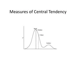
Positively Skewed Distribution Positively skewed: Mean and Median are to the right of the Mode
Negatively Skewed Distribution • Negatively Skewed: Mean and Median are to the left of the Mode
Levels of Measurement • Numbers are used to measure concepts • like fear of crime • support for the police or capital punishment. • The numbers are used as a code
Question? • Statistically, the question is • can we use mathematics to now analyze this code that we have established? • does it make sense to treat the numbers as such and perform arithmetic operations on them?
This code is called the level of measurement. It involves converting the concepts to numerical data. There are four categories and each have different attributes. However, the levels of measurement are cumulative, kind of like the steps on a ladder. You have to step on the first step to reach the second, and so on.
Each succeeding level automatically possesses the attributes of the level preceding it, plus another distinct one.
Levels of Measurement • Nominal level:involves the process of classifying data into categories. When we classify respondents by race or sex, we are using nominal measurement (i.e., 1 – Male, 2 – Female).
Nominal level measurement follows three basic rules: 1. The list of categories must be exhaustive and cover all the types of observations made. 2. The categories must be mutually exclusive. Each observation can only be classified in one way. 3. No ordering (>) is present in the list of categories. The order is arbitrary and no one classification is superior to another.
It does not make sense to discuss the mean (average) or median (midpoint) with nominal data. • It cannot be summed and divided, nor can it be ranked in order from highest to lowest. • Example: Table 3.2 from NCVS.
Here we see that the majority of the respondents are Male (52.1%). • Although everyone knows that women are smarter, we cannot say that the mutually exclusive categories of sex are in rank order, or can we say that one sex is “average.”
LEVELS OF MEASUREMENT • Ordinal level: Exists when we can also detect degrees of difference between the categories on the scale. The values of the variable indicate order or ranking. EXAMPLE:“Do you favor or oppose the death penalty for persons convicted of murder?” Choices:(1) Favor (2) Oppose (3) Neither (4) Don’t Know.
Transitivity • Ordinal level measurement requires transitivity. • If A is > B and B is > C, A must be greater than C or ordinal level measurement is not present. • “Favor” is > “Oppose,” “Oppose” is > “Neither,” “Neither is > “Don’t Know,” and “Favor” is > “Don’t Know.”
“Do you favor the death penalty for persons convicted of murder?”
LEVELS OF MEASUREMENT • Interval level: assumes that the difference between each item on the scale have equal units (or intervals) of measurement between them. It also assumes that this unit has a common recognized meaning.
LEVELS OF MEASUREMENT • Ratio level: Data possessing a natural zero point and organized into measures for which differences are meaningful. • Examples:A year is a common, constant unit of measurement. Before birth, a person is considered to have zero years of age. with ratio level measurement.
For example, analysis of the age of the respondents to the National Crime Survey revealed that the mean was 45.6 years. • The median or midpoint was 42. • The mode was also 42.
We can also compare groups of respondents according to their age. • The fourteen survey respondents were 44 (lets call them “Group A”) and twenty one respondents were 22 (Group B). • We draw the following conclusions about Respondents from Groups A and B:
They have different ages (Nominal Measurement). • Members of Group A are 22 years older than members of Group B (Ordinal and Interval Measurement). • Members of Group A are twice as old as members of Group B (Ratio Measurement).