Download
1 / 49
520 likes | 631 Views
Algorithms for Query Processing and Optimization. Chapter 15. Chapter Objectives. Introduction to the process of choosing a suitable execution strategy for processing a query. Chapter Outline. Introduction to Query Processing Translating SQL Queries into Relational Algebra

E N D
Algorithms for Query Processing and Optimization Chapter 15 ADBS: Query Opt.
Chapter Objectives • Introduction to the process of choosing a suitable execution strategy for processing a query. ADBS: Query Opt.
Chapter Outline • Introduction to Query Processing • Translating SQL Queries into Relational Algebra • Algorithms for External Sorting • Algorithms for the SELECT Operation • Algorithms for the JOIN Operation • Algorithms for the PROJECT Operation • Using Heuristics in Query Optimization • Using Selectivity and Cost Estimates in Query Optimization ADBS: Query Opt.
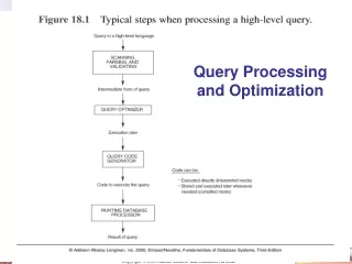
- Introduction to Query Processing ADBS: Query Opt.
- Translating SQL Queries into Relational Algebra … • Query block: the basic unit that can be translated into the algebraic operators and optimized. • A query block contains a single SELECT-FROM-WHERE expression, as well as GROUP BY and HAVING clause if these are part of the block. • Nested queries within a query are identified as separate query blocks. • Aggregate operators in SQL must be included in the extended algebra. ADBS: Query Opt.
… - Translating SQL Queries into Relational Algebra SELECT LNAME, FNAME FROM EMPLOYEE WHERE SALARY > ( SELECT MAX (SALARY) FROM EMPLOYEE WHERE DNO = 5); SELECT LNAME, FNAME FROM EMPLOYEE WHERE SALARY > C SELECT MAX (SALARY) FROM EMPLOYEE WHERE DNO = 5 πLNAME, FNAME(σSALARY>C(EMPLOYEE)) ℱMAX SALARY(σDNO=5 (EMPLOYEE)) ADBS: Query Opt.
- Algorithms for External Sorting … • External sorting: refers to sorting algorithms that are suitable for large files of records stored on disk that do not fit entirely in main memory, such as most database files. • Sort-Mergestrategy: starts by sorting small subfiles (runs) of the main file and then merges the sorted runs, creating larger sorted subfiles that are merged in turn. • Sorting phase: nR = ⌐(b/nB)¬ • Merging phase: dM = Min (nB-1, nR); nP = ⌐(logdM(nR))¬ nR: number of initial runs; b: number of file blocks; nB: available buffer space; dM: degree of merging; nP: number of passes. ADBS: Query Opt.
… - Algorithms for External Sorting Note: The above figure is now called Figure 15.2 in Edition 4 ADBS: Query Opt.
- The SELECT Operation • Examples: • (OP1): σSSN='123456789' (EMPLOYEE) • (OP2): σDNUMBER>5(DEPARTMENT) • (OP3): σDNO=5(EMPLOYEE) • (OP4): σDNO=5 AND SALARY>30000 AND SEX=F(EMPLOYEE) • (OP5): σESSN=123456789 AND PNO=10(WORKS_ON) ADBS: Query Opt.
- Algorithms for a Simple SELECT Operation … • S1. Linear search (brute force): Retrieve every record in the file, and test whether its attribute values satisfy the selection condition. • S2. Binary search: If the selection condition involves an equality comparison on a key attribute on which the file is ordered, binary search (which is more efficient than linear search) can be used. (See OP1). • S3. Using a primary index or hash key to retrieve a single record: If the selection condition involves an equality comparison on a key attribute with a primary index (or a hash key), use the primary index (or the hash key) to retrieve the record. ADBS: Query Opt.
… - Algorithms for a Simple SELECT Operation … • S4. Using a primary index to retrieve multiple records: If the comparison condition is >, ≥, <, or ≤ on a key field with a primary index, use the index to find the record satisfying the corresponding equality condition, then retrieve all subsequent records in the (ordered) file. • S5. Using a clustering index to retrieve multiple records: If the selection condition involves an equality comparison on a non-key attribute with a clustering index, use the clustering index to retrieve all the records satisfying the selection condition. • S6. Using a secondary (B+-tree) index: On an equality comparison, this search method can be used to retrieve a single record if the indexing field has unique values (is a key) or to retrieve multiple records if the indexing field is not a key. In addition, it can be used to retrieve records on conditions involving >,>=, <, or <=. (FOR RANGE QUERIES) ADBS: Query Opt.
… - Algorithms for a Complex SELECT Operation … • S7. Conjunctive selection: If an attribute involved in any single simple condition in the conjunctive condition has an access path that permits the use of one of the methods S2 to S6, use that condition to retrieve the records and then check whether each retrieved record satisfies the remaining simple conditions in the conjunctive condition. • S8. Conjunctive selection using a composite index: If two or more attributes are involved in equality conditions in the conjunctive condition and a composite index (or hash structure) exists on the combined field, we can use the index directly. ADBS: Query Opt.
… - Algorithms for a Complex SELECT Operation … • S9. Conjunctive selection by intersection of record pointers: This method is possible if secondary indexes are available on all (or some of) the fields involved in equality comparison conditions in the conjunctive condition and if the indexes include record pointers (rather than block pointers). Each index can be used to retrieve the record pointers that satisfy the individual condition. The intersection of these sets of record pointers gives the record pointers that satisfy the conjunctive condition, which are then used to retrieve those records directly. If only some of the conditions have secondary indexes, each retrieved record is further tested to determine whether it satisfies the remaining conditions. ADBS: Query Opt.
… - Implementing SELECT Operation • Whenever a single condition specifies the selection, we can only check whether an access path exists on the attribute involved in that condition. If an access path exists, the method corresponding to that access path is used; otherwise, the “brute force” linear search approach of method S1 is used. (See OP1, OP2 and OP3) • For conjunctive selection conditions, whenever more than one of the attributes involved in the conditions have an access path, query optimization should be done to choose the access path that retrieves the fewest records in the most efficient way . ADBS: Query Opt.
- Implementing the JOIN Operation … • Join (EQUIJOIN, NATURAL JOIN) • two–way join: a join on two files e.g. R A=B S • multi-way joins: joins involving more than two files. e.g. R A=B S C=D T • Examples (OP6): EMPLOYEE DNO=DNUMBER DEPARTMENT (OP7): DEPARTMENT MGRSSN=SSN EMPLOYEE ADBS: Query Opt.
… - Implementing the JOIN Operation … • J1. Nested-loop join (brute force): For each record t in R (outer loop), retrieve every record s from S (inner loop) and test whether the two records satisfy the join condition t[A] = s[B]. • J2. Single-loop join (Using an access structure to retrieve the matching records): If an index (or hash key) exists for one of the two join attributes — say, B of S — retrieve each record t in R, one at a time, and then use the access structure to retrieve directly all matching records s from S that satisfy s[B] = t[A]. ADBS: Query Opt.
… - Implementing the JOIN Operation … • J3. Sort-merge join: If the records of R and S are physically sorted (ordered) by value of the join attributes A and B, respectively, we can implement the join in the most efficient way possible. Both files are scanned in order of the join attributes, matching the records that have the same values for A and B. In this method, the records of each file are scanned only once each for matching with the other file—unless both A and B are non-key attributes, in which case the method needs to be modified slightly. • J4. Hash-join: The records of files R and S are both hashed to the same hash file, using the same hashing function on the join attributes A of R and B of S as hash keys. A single pass through the file with fewer records (say, R) hashes its records to the hash file buckets. A single pass through the other file (S) then hashes each of its records to the appropriate bucket, where the record is combined with all matching records from R. ADBS: Query Opt.
… - Implementing the JOIN Operation … • Factors affecting JOIN performance • Available buffer space • Join selection factor • Choice of inner VS outer relation ADBS: Query Opt.
-- Partition hash join … • Partitioning phase: • Each file (R and S) is first partitioned into M partitions using a partitioning hash function on the join attributes: R1 , R2 , R3 , ...... Rm and S1 , S2 , S3 , ...... Sm • A disk sub-file is created per partition to store the tuples for that partition. • Joining or probing phase: • Involves M iterations, one per partitioned file. Iteration i involves joining partitions Ri and Si. ADBS: Query Opt.
-- Partition hash join … • Assume Ri is smaller than Si. • Copy records from Ri into memory buffers. • Read all blocks from Si, one at a time and each record from Si is used to probe for a matching record(s) from partition Si. • Write matching record from Ri after joining to the record from Si into the result file. ADBS: Query Opt.
-- Partition hash join … • Cost analysis of partition hash join: • Reading and writing each record from R and S during the partitioning phase: (bR + bS), (bR + bS) • Reading each record during the joining phase: (bR + bS) • Writing the result of join: bRES Total Cost: 3* (bR + bS) + bRES ADBS: Query Opt.
- Algorithms for PROJECT Operation • <attribute list>(R) • If <attribute list> has a key of relation R, extract all tuples from R with only the values for the attributes in <attribute list>. • If <attribute list> does NOT include a key of relation R, duplicated tuples must be removed from the results. • Methods to remove duplicate tuples • Sorting • Hashing ADBS: Query Opt.
- Algorithm for SET operations … • Set operations: UNION, INTERSECTION, SET DIFFERENCE and CARTESIAN PRODUCT. • CARTESIAN PRODUCT of relations R and S include all possible combinations of records from R and S. The attribute of the result include all attributes of R and S. • Cost analysis of CARTESIAN PRODUCT • If R has n records and j attributes and S has m records and k attributes, the result relation will have n*m records and j+k attributes. • CARTESIAN PRODUCT operation is very expensive and should be avoided if possible. ADBS: Query Opt.
… - Algorithm for SET operations … • UNION (See Figure 15.3c) • Sort the two relations on the same attributes. • Scan and merge both sorted files concurrently, whenever the same tuple exists in both relations, only one is kept in the merged results. • INTERSECTION (See Figure 15.3d) • Sort the two relations on the same attributes. • Scan and merge both sorted files concurrently, keep in the merged results only those tuples that appear in both relations. • SET DIFFERENCE R-S (See Figure 15.3e) • (keep in the merged results only those tuples that appear in relation R but not in relation S.) ADBS: Query Opt.
- Combining Operations using Pipelining … • Motivation • A query is mapped into a sequence of operations. • Each execution of an operation produces a temporary result. • Generating and saving temporary files on disk is time consuming and expensive. • Alternative: • Avoid constructing temporary results as much as possible. • Pipeline the data through multiple operations - pass the result of a previous operator to the next without waiting to complete the previous operation. ADBS: Query Opt.
… - Combining Operations using Pipelining … • Example: For a 2-way join, combine the 2 selections on the input and one projection on the output with the Join. • Dynamic generation of code to allow for multiple operations to be pipelined. • Results of a select operation are fed in a "Pipeline" to the join algorithm. • Also known as stream-based processing. ADBS: Query Opt.
- Using Heuristics in Query Optimization … • Process for heuristics optimization • The parser of a high-level query generates an initial internal representation; • Apply heuristics rules to optimize the internal representation. • A query execution plan is generated to execute groups of operations based on the access paths available on the files involved in the query. • The main heuristic is to apply first the operations that reduce the size of intermediate results. E.g., Apply SELECT and PROJECT operations before applying the JOIN or other binary operations. ADBS: Query Opt.
… - Using Heuristics in Query Optimization … • Query tree: a tree data structure that corresponds to a relational algebra expression. It represents the input relations of the query as leaf nodes of the tree, and represents the relational algebra operations as internal nodes. • An execution of the query tree consists of executing an internal node operation whenever its operands are available and then replacing that internal node by the relation that results from executing the operation. ADBS: Query Opt.
… - Using Heuristics in Query Optimization … • Example: For every project located in ‘Stafford’, retrieve the project number, the controlling department number and the department manager’s last name, address and birthdate. SQL query: Q2: SELECT P.NUMBER,P.DNUM,E.LNAME, E.ADDRESS, E.BDATE FROM PROJECT AS P,DEPARTMENT AS D, EMPLOYEE AS E WHERE P.DNUM=D.DNUMBER AND D.MGRSSN=E.SSN AND P.PLOCATION=‘STAFFORD’; Relation algebra: PNUMBER, DNUM, LNAME, ADDRESS, BDATE (((PLOCATION=‘STAFFORD’(PROJECT)) DNUM=DNUMBER (DEPARTMENT)) MGRSSN=SSN (EMPLOYEE)) ADBS: Query Opt.
… - Using Heuristics in Query Optimization … Note: The above figure is now called Figure 15.4 in Edition 4 ADBS: Query Opt.
… - Using Heuristics in Query Optimization … Heuristic Optimization of Query Trees: • The same query could correspond to many different relational algebra expressions — and hence many different query trees. • The task of heuristic optimization of query trees is to find a final query tree that is efficient to execute. • Example: Q: SELECT LNAME FROM EMPLOYEE, WORKS_ON, PROJECT WHERE PNAME = ‘AQUARIUS’ AND PNMUBER=PNO AND ESSN=SSN AND BDATE > ‘1957-12-31’; ADBS: Query Opt.
… - Using Heuristics in Query Optimization … Note: The above figure is now called Figure 15.5 in Edition 4 ADBS: Query Opt.
… - Using Heuristics in Query Optimization … Note: The above figure is now called Figure 15.5(continued c, d) in Edition 4 ADBS: Query Opt.
… - Using Heuristics in Query Optimization … Note: The above figure is now called Figure 15.5(continued e) in Edition 4 ADBS: Query Opt.
-- General Transformation Rules for Relational Algebra Operations … • Cascade of s: A conjunctive selection condition can be broken up into a cascade (sequence) of individual s operations: s c1 AND c2 AND ... AND cn(R) = sc1 (sc2 (...(scn(R))...) ) • Commutativity of s: The s operation is commutative: sc1 (sc2(R)) = sc2 (sc1(R)) • Cascade of p: In a cascade (sequence) of p operations, all but the last one can be ignored: pList1 (pList2 (...(pListn(R))...) ) = pList1(R) • Commuting s with p: If the selection condition c involves only the attributes A1, ..., An in the projection list, the two operations can be commuted: pA1, A2, ..., An (sc (R)) = sc (pA1, A2, ..., An (R)) ADBS: Query Opt.
… -- General Transformation Rules for Relational Algebra Operations … • Commutativity of ( and x ): The operation is commutative as is the x operation: R C S = S C R; R x S = S x R • Commuting s with (or x ): If all the attributes in the selection condition c involve only the attributes of one of the relations being joined—say, R—the two operations can be commuted as follows : sc ( R S ) = (sc (R)) S Alternatively, if the selection condition c can be written as (c1 and c2), where condition c1 involves only the attributes of R and condition c2 involves only the attributes of S, the operations commute as follows: sc ( R S ) = (sc1 (R)) (sc2 (S)) ADBS: Query Opt.
… -- General Transformation Rules for Relational Algebra Operations … • Commuting p with (or x ): Suppose that the projection list is L = {A1, ..., An, B1, ..., Bm}, where A1, ..., An are attributes of R and B1, ..., Bm are attributes of S. If the join condition c involves only attributes in L, the two operations can be commuted as follows: pL ( R C S ) = (pA1, ..., An (R)) C (pB1, ..., Bm (S)) If the join condition c contains additional attributes not in L, these must be added to the projection list, and a final p operation is needed. ADBS: Query Opt.
… -- General Transformation Rules for Relational Algebra Operations … • Commutativity of set operations: The set operations υ and ? are commutative but – is not. • Associativity of , x, υ, and ∩ : These four operations are individually associative; that is, if q stands for any one of these four operations (throughout the expression), we have: ( R q S ) q T = R q ( S q T ) • Commuting s with set operations: The s operation commutes with υ , ∩ , and –. If q stands for any one of these three operations, we have sc ( R q S ) = (sc (R)) q (sc (S)) ADBS: Query Opt.
… -- General Transformation Rules for Relational Algebra Operations … • The p operation commutes with υ. pL ( R υ S ) = (pL (R)) υ (pL (S)) • Converting a (s, x) sequence into : If the condition c of a s that follows a x Corresponds to a join condition, convert the (s, x) sequence into a as follows: (sC (R x S)) = (R C S) • Other transformations ADBS: Query Opt.
-- Outline of a Heuristic Algebraic Optimization Algorithm … • Using rule 1, break up any select operations with conjunctive conditions into a cascade of select operations. • Using rules 2, 4, 6, and 10 concerning the commutativity of select with other operations, move each select operation as far down the query tree as is permitted by the attributes involved in the select condition. • Using rule 9 concerning associativity of binary operations, rearrange the leaf nodes of the tree so that the leaf node relations with the most restrictive select operations are executed first in the query tree representation. • Using Rule 12, combine a cartesian product operation with a subsequent select operation in the tree into a join operation. ADBS: Query Opt.
… -- Outline of a Heuristic Algebraic Optimization Algorithm • Using rules 3, 4, 7, and 11 concerning the cascading of project and the commuting of project with other operations, break down and move lists of projection attributes down the tree as far as possible by creating new project operations as needed. • Identify subtrees that represent groups of operations that can be executed by a single algorithm. ADBS: Query Opt.
-- Summary of Heuristics for Algebraic Optimization • The main heuristic is to apply first the operations that reduce the size of intermediate results. • Perform select operations as early as possible to reduce the number of tuples and perform project operations as early as possible to reduce the number of attributes. (This is done by moving select and project operations as far down the tree as possible.) • The select and join operations that are most restrictive should be executed before other similar operations. (This is done by reordering the leaf nodes of the tree among themselves and adjusting the rest of the tree appropriately.) ADBS: Query Opt.
- Cost Based Optimization (CBO) • Cost-based query optimization: Estimate and compare the costs of executing a query using different execution strategies and choose the strategy with the lowest cost estimates • In heuristic query optimization parameters such as the size of the operand tables is not considered. • Issues in cost based optimization • Cost function • Number of execution strategies to be considered ADBS: Query Opt.
-- Using Selectivity and Cost Estimates in CBO … • Cost Components for Query Execution • Access cost to secondary storage • Storage cost • Computation cost • Memory usage cost • Communication cost Note: Different database systems may focus on different cost components. ADBS: Query Opt.
… -- Using Selectivity and Cost Estimates in CBO • Catalog Information Used in Cost Functions • Information about the size of a file • number of records (tuples) (r), • record size (R), • number of blocks (b) • blocking factor (bfr) • Information about indexes and indexing attributes of a file • Number of levels (x) of each multilevel index • Number of first-level index blocks (bI1) • Number of distinct values (d) of an attribute • Selectivity (sl) of an attribute • Selection cardinality (s) of an attribute. (s = sl * r) ADBS: Query Opt.
--- Examples of Cost Functions for SELECT … • S1. Linear search (brute force) approach CS1a = b; For an equality condition on a key, CS1a = (b/2) if the record is found; otherwise CS1a = b. • S2. Binary search: CS2 = log2b + ┌(s/bfr) ┐–1 For an equality condition on a unique (key) attribute, CS2 =log2b • S3. Using a primary index (S3a) or hash key (S3b) to retrieve a single record CS3a = x + 1; CS3b = 1 for static or linear hashing; CS3b = 1 for extendible hashing; ADBS: Query Opt.
… --- Examples of Cost Functions for SELECT … • S4. Using an ordering index to retrieve multiple records: For the comparison condition on a key field with an ordering index, CS4 = x + (b/2) • S5. Using a clustering index to retrieve multiple records: CS5 = x + ┌ (s/bfr) ┐ • S6. Using a secondary (B+-tree) index: For an equality comparison, CS6a = x + s; For an comparison condition such as >, <, >=, or <=, CS6a = x + (bI1/2) + (r/2) ADBS: Query Opt.
… --- Examples of Cost Functions for SELECT • S7. Conjunctive selection: Use either S1 or one of the methods S2 to S6 to solve. For the latter case, use one condition to retrieve the records and then check in the memory buffer whether each retrieved record satisfies the remaining conditions in the conjunction. • S8. Conjunctive selection using a composite index: Same as S3a, S5 or S6a, depending on the type of index. ADBS: Query Opt.
End ADBS: Query Opt.