Download
1 / 23
230 likes | 238 Views
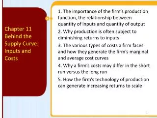
CHAPTER 8 Inputs and Costs. Definitions:. A production function is the relationship between the quantity of inputs a firm uses and the quantity of output it produces. A fixed input is an input whose quantity is fixed and cannot be varied. (Short run)

E N D
CHAPTER 8 Inputs and Costs
Definitions: A production function is the relationship between the quantity of inputs a firm uses and the quantity of output it produces. A fixed input is an input whose quantity is fixed and cannot be varied. (Short run) A variable input is an input whose quantity the firm can vary. (Short run)
The long run is the time period in which ALL inputs can be varied. The short run is the time period in which at least one input is fixed. The total product curve shows how the quantity of output as dependent upon the quantity of the variable input.
Production Function and TP Curve for George and Martha’s Farm Although the total product curve in the figure slopes upward along its entire length, the slope isn’t constant: as you move up the curve to the right, it flattens out due to changing marginal product of labor.
Marginal Product of Labor The marginal product of an input is the additional quantity of output that is produced by using one more input unit.
Diminishing Returns to an Input There are diminishing returns to an input when an increase in the quantity of that input, holding the levels of all other inputs fixed, leads to a decline in the marginal product of that input.
Marginal Product of Labor Curve Here, the first worker employed generates an increase in output of 19 bushels, the second worker generates an increase of 17 bushels, and so on…
Panel (a) shows two total product curves for George and Martha’s farm. With more land, each worker can produce more wheat. So an increase in the fixed input shifts the total product curve up from TP10 to TP20. This shift also implies that the marginal product of each worker is higher when the farm is larger. As a result, an increase in acreage also shifts the marginal product of labor curve up from MPL10 to MPL20.
From the Production Function to Cost Curves A fixed cost is a cost that does not depend on the quantity of output produced. It is the cost of the fixed input. A variable cost is a cost that depends on the quantity of output produced. It is the cost of the variable input.
Total Cost Curve The total cost of producing a given quantity of output is the sum of the fixed cost and the variable cost of producing that quantity of output. TC = FC + VC The total cost curve becomes steeper as more output is produced due to diminishing returns.
Total Cost and Marginal Cost Curves for Ben’s Boots Why is the marginal cost curve upward sloping? Because there are diminishing returns to inputs in this example. As output increases, the marginal product of the variable input declines. This implies that more and more of the variable input must be used to produce each additional unit of output as the amount of output already produced rises. And since each unit of the variable input must be paid for, the cost per additional unit of output also rises.
Average Cost Average total cost, often referred to simply as average cost, is total cost divided by quantity of output produced. ATC = TC/Q Average fixed cost is the fixed cost per unit of output. AFC = FC/Q Average variable cost is the variable cost per unit of output. AVC = VC/Q
Marginal Cost and Average Cost Curves for Ben’s Boots The bottom of the U curve is at the level of output at which the marginal cost curve crosses the average total cost curve from below. Is this an accident? No!
The Relationship Between the Average Total Cost and the Marginal Cost Curves When marginal cost equals average total cost, we must be at the bottom of the U, because only at that point is average total cost neither falling nor rising.
More Realistic Cost Curves Marginal cost curves do not always slope upward. The benefits of specialization of labor can lead to increasing returns at first represented by a downward-sloping marginal cost curve. Once there are enough workers to permit specialization, however, diminishing returns set in.
Short-Run versus Long-Run Costs In the short run, fixed cost is completely outside the control of a firm. But all inputs are variable in the long run: The firm will choose its fixed cost in the long run based on the level of output it expects to produce.
Choosing the Level of Fixed Cost for Ben’s Boots There is a trade-off between higher fixed cost and lower variable cost for any given output level, and vice versa. But as output goes up, average total cost is lower with the higher amount of fixed cost.
The long-run average total cost curve shows the relationship between output and average total cost when fixed cost has been chosen to minimize average total cost for each level of output. The Long-Run Average Total Cost Curve
Economies and Diseconomies of Scale • There are economies of scale when long-run average total cost declines as output increases. • There are diseconomies of scale when long-run average total cost increases as output increases. • There are constant returns to scale when long-run average total cost is constant as output increases.