Download
1 / 25
260 likes | 341 Views
Basic Data Analysis Using R. Xiao He. Agenda. Data cleaning (e.g., missing values) Descriptive statistics t -tests ANOVA Linear regression. Data visualization. Agenda. Data cleaning (e.g., missing values) Descriptive statistics t -tests ANOVA Linear regression. 1. Data cleaning.

E N D
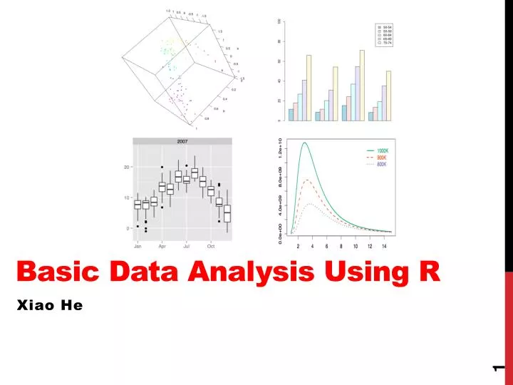
Basic Data Analysis Using R Xiao He
Agenda • Data cleaning (e.g., missing values) • Descriptive statistics • t-tests • ANOVA • Linear regression Data visualization
Agenda • Data cleaning (e.g., missing values) • Descriptive statistics • t-tests • ANOVA • Linear regression
1. Data cleaning NOTE: You may have coded missing values using other notations. For example, some researchers/programs use -99 or -999 to denote missing values. If that is the case, you need to check for missing values using other methods that won’t be covered here. • NA and NaN: • 1. NA(Not Available): missing values. • a). Represented in the form of NA, or in the form of <NA>. • 2. NaN(Not a number): when an arithmetic operation returns a non-numeric result: e.g., in R, 0/0 gives you NaN.
1. Data cleaning • NA and NaN: • 3. Deal with NA and NaN? • a). Check how many cases (rows) do NOT have NAor NaN: • complete.cases() • #Returns Booleans (TRUE, FALSE). TRUE means no missing • #value (in a given row), and FALSE means there is at • #least one missing value. • b). Remove cases with NAor NaN: • na.omit() • #return a data object with NA and NaN removed. For data • #frames, an entire row will be removed if it contains NA • #or NaN. • c). More sophisticated ways of dealing with NA(covered by Addie’s workshop in two weeks)
Agenda • Data cleaning (e.g., missing values) • Descriptive statistics • t-tests • ANOVA • Linear regression
2. Descriptive statistics • Help you diagnose potential problems w/ data entry or collection: • Were any values entered incorrectly? e.g., survey study using 1 – 5 Likert scale, but when you checked the range of your data, you found that the maximum value in your dataset was 7. • Any strange responses? e.g., Did your participants give you any odd responses? • Help you get a sense of how your data are distributed. • Extreme values (outliers) • Non-normality • Skewness • Unequal variance
2. Descriptive statistics • Compute individual descriptive statistics • Location: • mean(x, trim) • median(x) • Dispersion • var(x) • sd(x) • range(x); min(x); max(x) • IQR(x)
2. Descriptive statistics • Compute a set of descriptive statistics • Use the function summary(). • function describe() in the package `psych`.
Agenda • Data cleaning (e.g., missing values) • Descriptive statistics • t-tests • ANOVA • Linear regression
3. T tests • t.test() • t.test(x, y = NULL, • alternative=c("two.sided", "less", "greater”), • mu = 0, paired = FALSE, var.equal = FALSE, • conf.level = .95) • One-sample t-test:
3. T tests • t.test() • t.test(x, y = NULL, • alternative=c("two.sided", "less", "greater”), • mu = 0, paired = FALSE, var.equal = FALSE, • conf.level = .95) • One-sample t-test: Suppose someone hypothesized that the mean undergrad age was 19.75. Let’s test whether the mean age was significantly different from 19.75. • H0: mu0 = 19.75 • H1: mu0 ≠ 19.75
3. T tests • t.test() • t.test(x, y = NULL, • alternative=c("two.sided", "less", "greater”), • mu = 0, paired = FALSE, var.equal = FALSE, • conf.level = .95) • Independent t-test: • Let’s test whether the mean height of female students is significantly different from the mean height of male students • H0: muFemale = muMale • H1: muFemale≠ muMale
3. T tests formula = Y ~ X Y: outcome variable (e.g., height) X: 2 level grouping variable (e.g., Sex) • t.test() • t.test(x, y = NULL, • alternative=c("two.sided", "less", "greater”), • mu = 0, paired = FALSE, var.equal = FALSE, • conf.level = .95) • t.test(formula, data,…) • Independent t-test: • Let’s test whether the mean height of female students is significantly different from the mean height of male students • H0: muFemale = muMale • H1: muFemale≠ muMale
3. T tests • t.test() • t.test(x, y = NULL, • alternative=c("two.sided", "less", "greater”), • mu = 0, paired = FALSE, var.equal = FALSE, • conf.level = .95) • t.test(formula, data,…) • Paired t-test: • Let’s test whether the mean Writing hand span (Wr.Hnd) and the mean Non-writing hand span (NW.Hnd) differ significantly. • H0: muWr.Hnd = muNW.Hnd • H1: muWr.Hnd≠ muNW.Hnd
Agenda • Data cleaning (e.g., missing values) • Descriptive statistics • t-tests • ANOVA • Linear regression
4. ANOVA • aov() • aov(formula, data) • One-way ANOVA: • Suppose we are interested in whether the mean pulse rates differ amongst people of different exercise statuses. • H0: muNone = muSome = muFreq • H1: Not all groups are equal.
We will import a new dataset and will use it for the next exercise. • hsb2 <- read.table("http://www.ats.ucla.edu/stat/r/faq/hsb2.csv", sep=",", header=TRUE)
4. ANOVA • aov() • aov(formula, data) • Two-way ANOVA: • The formula/model for factorial ANOVA (take 2 way interaction for example) is specified as follows: • Y ~ X1 * X2 which is equivalent to Y ~ X1 + X2 + X1:X2 • Suppose we are interested the main effects of raceand schtyp(school type) as well as the interaction effect between the two variables on read. The formula/model can be specified as: • read ~ as.factor(race) * as.factor(schtyp) Why do we do this?
Note • In R, by default, ANOVA results are based on Type 1 (“sequential”) Sum of Squares. Some other programs report Type 3 SS (SPSS) or both Type 1 and Type 3 (SAS). The Type 3 SS for each term is calculated given all other terms are in the model.
Agenda • Data cleaning (e.g., missing values) • Descriptive statistics • t-tests • ANOVA • Linear regression
Let’s import a new dataset • expenditure <- read.table("http://dornsife.usc.edu/assets/sites/210/docs/GC3/educationExpenditure.txt", sep=",", header=TRUE)
5. Linear regression • lm() • lm(formula, data) • education: Per-capita education expenditures, dollars. • income:Per-capita income, dollars. • young: Proportion under 18, per 1000. • urban: Proportion urban, per 1000. • Simple linear regression • formula = Y ~ X • Suppose we are interested in testing the regression of per-capita education expenditure on per-capita income, the model should be specified as: • formula = education ~ income
5. Linear regression • lm() • lm(formula, data) • education: Per-capita education expenditures, dollars. • income:Per-capita income, dollars. • young: Proportion under 18, per 1000. • urban: Proportion urban, per 1000. • Multiple regression • formula = Y ~ X1 + X2 + … + Xp • Suppose we are interested in testing the regression of education on income, young, and urban, the model should be specified as: • formula = education ~ income + young + urban