Download

1 / 49
540 likes | 795 Views
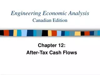
IE2311 Engineering Economic Analysis. Engineering Costs and Cost Estimating Department of Industrial Engineering Himlona Palikhe , PhD Candidate. Objectives.

E N D
IE2311 Engineering Economic Analysis Engineering Costs and Cost Estimating Department of Industrial Engineering Himlona Palikhe, PhD Candidate
Objectives • Learn basic cost accounting terms and cost estimation methods, as a foundation for the rest of this course and engineering economic analysis in real life.
Cost Estimation in Engineering Economy • “Cost” estimation is necessary for almost any engineering economic analysis in real life • Sometimes cost estimation is the entire analysis • Unlike real life, in this course, costs are often given in the problem
Major topics to be covered • Calculating total cost and profit • Identifying real vs. accounting costs • Cost estimation methods – e.g., power sizing and learning curves
Calculating total cost and profit All organizations are vitally concerned about the following equation: Profit = Revenue (Sales + Investments) – Expenses (Cost of doing business) The goal is: Maximizing Profit (Profit >= 0) For not-for-profit organizations, the goal is: Profit = 0
Calculating total cost and profit For any product, project or process, there are two basic types of costs involved in the total cost of the endeavor: • Fixed Cost = Pay regardless of production levels – setup costs • Variable Cost = Per unit cost – only charged when we produce a unit
Example #1 A student organization planning a one-day conference is trying to figure out how much to charge each participant. The following costs have been identified. Classify each as fixed or variable: • Auditorium rental • Box lunches • Audio-visual setup for the auditorium • Conference brochures • Workbooks for participants
Calculating total cost and profit Based on the previous slides, we can also define: • Total Cost = TFC + TVC = F + Vx • (where x = production quantity) • Average Cost = TC/x = (F+Vx)/x = F/x + V • Marginal Cost = Cost to produce one additional unit – typically just V
Example #2 Based on the estimates, define the equation for the total cost of the conference: • Auditorium rental - $130 • Meals - $8 • Audio-visual setup for the auditorium - $50 • Conference brochures - $45 • Workbooks for participants - $12 • TC = F + Vx = (130+50+45) + (8+12)x • = 225 + 20x
Calculating total cost and profit Cost is only one side of the profit equation: • Total Revenue = Price * Products sold = Px • Breakeven Point • TR = TC • Px = F + Vx • (P – V)x = F • x = F/(P – V)
Calculating total cost and profit We can also define: • Profit Region • = TR > TC • Loss Region • = TR < TC Profit Loss
Example #3 The student organization is trying to determine whether $35 per participant would be a reasonable charge. If this price is used, what is the breakeven point? Does this price seem reasonable? Why or why not?
Example #3 Cont. Solution: • X = F/(P-V) = 225/(35-20) = 15 • TR = TC • 35x = 225 + 20x • 15x = 225 • x = 15 • May be lower the price to increase attendance
Breakeven Graph What is the minimum number of units the organization should produce to generate a profit?
Identifying real vs. accounting costs In engineering economy, sometimes the “costs” we encounter don’t represent real transactions. • Cash Cost = money actually changing hands/location (money moving) • Book Cost = due to accounting convention no money is actually moving eg. Depreciation, some overhead costs However, many “fake” costs are still part of the analysis. Why? If it is production specific “overhead”, specific to project or for tax purposes and depreciation.
Example #4 A company is considering whether to outsource its printing or retain its internal printing department. The following analysis has been performed: • Cost for 30,000 copies external = $688 • Cost for 30,000 copies internal = $813, based on: • Direct labor: $228 • Materials and supplies: $294 • Re-allocated organizational overhead: $291 Which alternative should be selected?
Identifying real vs. accounting costs Two other important cost terms • Sunk Cost = money invested in the past (outside our time frame of interest) • Opportunity Cost = benefit forgone to select the current alternative Which one should we typically ignore?
Example #5 Suppose you purchased a used Toyota Corolla three years ago. You are trying to decide whether to sell the Corolla. Which of the following represent opportunity costs? • Price you paid to purchase the Toyota Corolla - • Your storage and maintenance costs to date - • Current list price of a newer model Camry you are considering – cost of competing alternative • Current blue book value of the Corolla -
Example #6 Your company wins a contract for 3 million parts with the following manufacturing costs: • Material: $0.40/unit • Direct labor: $0.15/unit • Initial investment: $500,000 Halfway through product, you learn that a new production method is available, with the following costs: • Material: $0.34/unit • Direct labor: $0.10/unit • Additional investment: $100,000 In both situations, overhead is 2.5 times the direct labor costs. Should the new production method be adopted?
Other frequently encountered costs • Recurring Cost = Costs that occur at set intervals (repeating) A, G • Nonrecurring Cost = one-time costs P, F • Lifecycle Cost = looking at costs from conceptual design to product disposal (cost from birth to death) • Incremental Cost = Cost of 1 alternative over another • ROR, B/C
Project Life Cycle Go or No Go
Example #7 Coating for a plastic water bottle:
Solution • Compare on cost and find Breakeven point, preferred cost range for each if both are equally likely. • Process 1 = Process 2 • $10.8M + $0.059x = $7.5M + $0.067x • (10.8-7.5)M = (0.067-0.059)x • 3.3M = 0.008x • X = 3.3/0.008 = 412.5M • Preferred range for Process 1: 413M or above • Preferred range for Process 1: 412M or below
Cost Estimating • Rough: gut level, inaccurate • Semi-detailed: based on historical records, reasonably sophisticated and accurate • Detailed: based on detailed specifications and cost models, very accurate • Why don’t we always use detailed estimates?
Estimating Models • Per Unit and Segmenting • Cost Indexes where Ct = estimated cost at present time t C0 = cost at previous time t0 It = index value at time t I0= index value at time t0
Example #8 An engineer wants to estimate the cost of skilled labor for a construction project. The following information is available: • A similar project was completed five years ago at a cost of $360,000 • The ENR skilled labor index at the time of the previous project was 3496.27 • The ENR skilled labor index is 4038.44 today
Solution • = $360,000 (4038.44/3496.27) • = $415,825.55
Estimating Models • Power Sizing • Learning Curve • Triangulation
Power-sizing • Scale equipment costs up or down based on known costs and power-sizing exponents x: power-sizing exponent
Example #9 A 10,000-cubic-feet centrifugal blower costs $120,000. Estimate the cost for a 15,000 cubic feet centrifugal blower. Cost of equipment A = = = $152,431
Learning Curves • Production rate increases as volume increases
Example #10 If the first unit of a product took 32 minutes to produce and the learning curve rate is 80%, how much time will the 100th unit take? b = log 0.8/log 2 = -0.322 = 7.264 minutes
Example #11 If the time required for the first and eighth units are 10 hours and 7.29 hours respectively in a production operation, determine the learning curve percentage for this operation.
Example #11 Contd. • Solving for k • b = logk/log2 • log0.729/log8 = logk/log2 • logk = (log0.729/log8)log2
Cash Flow Diagrams • "The receipts and disbursements in a given time interval are referred to as cash flow, with the positive cash flows usually representing receipts and negative cash flows representing disbursements." Net Cash Flow = Receipts - Disbursements
Cash Flow Diagrams (Cont …) • Cash Flow Diagram: is simply a graphical representation of cash flows drawn on a time scale. • End of the Year Convention: a simplifying convention where all cash flow occurs at the end of the interest period.
Cash Flow Diagrams (Cont…) • CFD summarize how costs & benefits occur over time • CFD illustrates the size, sign, and timing of individual cash flows • Components of CFD • A segmented time-based horizontal line, divided into time units • A vertical arrow representing a cash flow is added at the time it occurs • Arrow pointing down for costs and up for benefits Newnan, D.G., J.P. Lavelle, and T.G. Eschenbach (2008). Engineering Economic Analysis, (10th ed.), Oxford University Press, Oxford.
1 2 5 4 3 0 Cash Flow Diagrams • Positive $100 • Negative $100 • Positive $100 • Negative $150 • Negative $150 • Positive $50 100 • Time line • Costs and benefits shown 50 0 -100 -150 Newnan, D.G., J.P. Lavelle, and T.G. Eschenbach (2008). Engineering Economic Analysis, (10th ed.), Oxford University Press, Oxford.
Example 12 • Consider the situation where P = $2,000 is borrowed and F is to be found after 5 years. • Construct the cash-flow diagram for this case, assuming an interest rate of 12% per year.
Solution • Figure 1.3 presents the cash-flow diagram.
Example 13 • If you start now and make five deposits of A = $1,000 per year in a 17%-per-year account, how much money will be accumulated (and can be withdrawn) immediately after you have made the last deposit? • Construct the cash-flow diagram.
Solution • The cash flows are shown below
Cash Flow – Categories • First cost: expenses to build or to buy and install • Operations and maintenance (O&M): annual expense, such as electricity, labor, and minor repairs • Salvage value: receipt at project termination for sale or transfer of the equipment • Revenues: annual receipts due to sale of products or services • Overhaul: major capital expenditure that occurs during the asset’s life Newnan, D.G., J.P. Lavelle, and T.G. Eschenbach (2008). Engineering Economic Analysis, (10th ed.), Oxford University Press, Oxford.
Cash Flow Diagrams • CFD shows when all cash flows occur • In a CFD, the end of period t is the same time as the beginning of period t+1 • Rent, lease, and insurance payments are usually treated as beginning-of-period cash flows • O&M, salvage, revenues, and overhauls are assumed to be end-of-period cash flows • The choice of time 0 is arbitrary Newnan, D.G., J.P. Lavelle, and T.G. Eschenbach (2008). Engineering Economic Analysis, (10th ed.), Oxford University Press, Oxford.
Cash Flow Logic • Question: Would you rather • Receive $1,000 today or • Receive $1,000 10 years from today? • Answer: TODAY of course! • Why? • I could invest $1000 today to make more money • I could buy a lot of stuff today with $1000 • Who knows what will happen in 10 years? • What if you could receive $ 3,000 10 years from today? Newnan, D.G., J.P. Lavelle, and T.G. Eschenbach (2008). Engineering Economic Analysis, (10th ed.), Oxford University Press, Oxford.
4 4 2 2 3 3 1 1 0 0 5 5 Cash Flow – Example 14 • To purchase a new $30,000 machine, • Pay the full price now minus a 3% discount or • Pay $5000 now; $8000 at the end of year 1; and $6000 at the end of each of the next 4 years Pay in full Pay in 5 years $5,000 $29,100 $6,000 $8,000 Newnan, D.G., J.P. Lavelle, and T.G. Eschenbach (2008). Engineering Economic Analysis, (10th ed.), Oxford University Press, Oxford.
2 1 0 Cash Flow – Example 15 • To repay a loan of $1,000 at 8% interest in 2 years • Repay half of $1000 plus interest at the end of each year $1000 $540 $580 Newnan, D.G., J.P. Lavelle, and T.G. Eschenbach (2008). Engineering Economic Analysis, (10th ed.), Oxford University Press, Oxford.
Information Updates • Assignment for Next Class: • Quiz 1 on Friday • Read Chapter 3 before class • Do Chapter 2 Homework Problems • My office hours • MWF 4:00 pm – 5:00 p.m. IE 210B