Download

1 / 52
520 likes | 631 Views
Detecting Outliers in IoT Data Streams. S ystemX Seminar 14 March 2019. Vassilis Christophides INRIA Paris ( MiMove ) vassilis.christophides@inria.fr Mike Giannoulis & Theodoros Marios Giakoumakis Computer Science Department, University of Crete. Universality of IoT Technology.

E N D
Detecting Outliers in IoT Data Streams SystemX Seminar 14 March 2019 • VassilisChristophides • INRIA Paris (MiMove) vassilis.christophides@inria.fr • Mike Giannoulis & TheodorosMariosGiakoumakis • Computer Science Department, University of Crete
Universality of IoT Technology Smart Energy Smart Transport & Logistics Smart Buildings Smart Agriculture Public Safety Smart Homes & Cities Smart Factories Smart Health Smart Retail • "From autonomous cars to intelligent personal assistants, data is the lifeblood of a rapidly growing digital existence – opening up opportunities previously unimagined by businesses“ IDC
Massive Size and Growth of IoT 1021 https://www.slideshare.net/IoTBruce/iot-meets-big-data-the-opportunities-and-challenges-by-syed-hoda-of-parstream EMC IDC digital universe of opportunities • By 2025, about 25% of all data will be realtime in nature out of which 95% of it will be generated by IoT!
IoT Data: Sensing the Physical World! 1018 • IoT data is becoming soon “mega” big(i.e. billions of connected Things) • 44EB / months corresponds to ~ 100M hard disks • Processing 44 EB with 100M servers would still take > one hour • IoT “data in motion” as opposed to traditional “data at rest” • Data speed is bound by the sensing frequency and connectivity • Data throughput (vs processing) has become the limiting factor! • High variety datae.g., from heterogeneous Things, embedded in the environment or wearable by persons • High veracity data(dropped or unlivable) as IoT data quality depends on how Things are used and connected in the wild • High variability dataasThings frequently change behavior dynamically and in ways that are not fully known in advance • Data security, privacy, etc. even more important!
IoT Data Analytics Anomaly Detection • Use Cases • Real-time monitoring and control • Failure detection and predictive maintenance • Malicious cyber activity detection • Product life-cycle management • Operational efficiency, optimization, self-adaptation • Batch and Online Techniques • Descriptive Analytics: aggregation and statistics • Predictive Analytics: Supervised, Semi-Supervised, Unsupervised • Data series analytics: Spatiotemporal • Domain and data type specific: Signal processing
Real Time Anomaly Detection Define alerts, predict faults, detect intrusions & threats
A Fog/Edge Computing Architecture large compute storage B. Tang, Z. Chen, G. Hefferman, T. Wei, H. He, Q. Yang. A Hierarchical Distributed Fog Computing Architecture for Big Data Analysis in Smart Cities. ASE BD&SI 2015 offline larger compute limited storage online limited compute storage real time
So to Recap • The Internet of Things Is more About Data, than Things! • data in motion usually with spatiotemporal semantics • produced by several, distributed, heterogeneous devices • in the wild, hence data prone to errors and noise • Low-latency, privacy-awareIoT data processing in post-cloud architectures • Edge/fog computing for effectively and efficiently ingesting and analyzing data whenandwhereit is needed • Real time IoT Data Analytics requires data streams support • Limited ground truth calls for unsupervised techniques
Data Anomalies • What are anomalies? • “An outlier is an observationin a dataset that appears to be inconsistent with the remainder of that dataset” [Johnson 1992] • “An outlier is an observation that deviatesso much from other observations as to arouse suspicion that it was generated by a different mechanism” [Hawkins 1980] • Anomaly, or outlier, or deviation, or noveltydetection, aims to measure whether a data point (or a subset) considerably differs than the remainder of the data points • On a scatter plot of the data, they lie far away from other data • Anomalies = Outliers + Novelties http://www.kdd.org/kdd2016/topics/view/outlier-and-anomaly-detection
Cause of Data Anomalies • Errors in the data collection or measurement process • Because of human error(intentional or not), a problem with a measuring device or the presence of noise • Insights extracted from “dirty data” are probably erroneous and thus the decisions to be made are likely unsound (e.g., incur a high rate of false positives and false negatives) • Changes in the “data generation” process, e.g. some given statistical process(not an error, novelties in data) • Abnormal data deviate from this generating mechanismbecause it is of a different type • Novel class of observations provide valuable insights
Types of Anomalies Point Anomaly Detection Data point anomalous w.r.t. to the rest of the data Data point anomalous in a specific context; also referred to as conditional anomalies • Requires a notion of context • the spatial or temporal neighborhood Contextual Anomaly Detection A group of data points is anomalous; the individual points within a group are not anomalous by themselves • Requires a relationship among data instances • Sequential data • Spatial data • Graph data • that is, a single object isunsuspicious while a collection of similar objects becomesspurious Group Anomaly Detection Chandola, V., Banerjee, A., & Kumar, V. (2009). Anomaly detection: A survey. ACM Computing Surveys, 41(3), 1–58.
Scope of Anomaly Detection Methods global local o1 o3 micro-cluster N1 O4 global o2 N2 • Swamping: wrongly identifying normal instances as anomalies when normal instances are too close to anomalies • Masking : an anomaly is close to another point, anomalous or not false positives false negatives M. Goldstein, S. UchidaAComparative Evaluation of Unsupervised Anomaly Detection Algorithms for Multivariate Data. PLoS One. 2016;11(4)
Example: Most Unusual Objects? battery screw https://www.slideshare.net/mlvlc/l14-anomaly-detection bead block box key knob penny dime eraser
Example: How to Distinguish Objects? https://www.slideshare.net/mlvlc/l14-anomaly-detection
High-Dimensional Data: Example https://www.slideshare.net/mlvlc/l14-anomaly-detection round skinny
Multi-Dimensional Anomaly Detection • Anomaly detection in multi-dimensionaldatasets reveals more accurate behavior of the data but at the same time poses various challenges http://wikistat.fr/pdf/st-m-app-anomalies.pdf
Multi-Dimensional Anomaly Detection • Space concentration of distances: feature-wise distances of i.i.d. data samples approximately converge to a normal distribution • The number of feature subspaces grows exponentially with the increasing dimensionality of data: data density functions not easily computed • Data-snooping bias: given enough features, at least one feature subspace can be found for each data point such that it appears as an anomaly D. L. Donoho, “High-dimensional data analysis: The curses and blessings of dimensionality,” AMS Math Challenges Lecture, pp. 1–32, 2000.
Anomaly Detection Methods Machine Learning Statistical Parametric Non Parametric Semi-Supervised Supervised Unsupervised Goldstein M, Uchida S (2016) A Comparative Evaluation of Unsupervised Anomaly Detection Algorithms for Multivariate Data. PLOS ONE 11(4) HBOS IQR Gaussian Classification Clustering based Nearest Neighbor based Ensemble based One class SVM Subspace based PSVM Isolation Forest Tree-based Distance-based Density based CBLOF– uCBLOF Kernel-based Neural Network-based SVDD Half-Space rPCA DB-Outlier COD - MCOD Hoeffding LOF QSSVM Multi-instance Learning CMGOS LOCI kth-NN CESVM RRCF ABOD Storm Streaming Algorithms
Random Trees • Build a decision tree from a random data subsample F T https://www.slideshare.net/mlvlc/l14-anomaly-detection T F • Partition feature space using axis-parallel subdivisions • Select the splitfeatureA, randomly and uniformly • Select the splitvalueVA, uniformly as the min(A)+(max(A)–min(A))*rand(1) • Grow a random tree until each data point is in its own leaf or the tree reaches a maximum height
Isolation Forest [Liu et al. 2008] • To score a data point, find the height of the leaf node • The smaller the height the more anomalous is the data https://www.slideshare.net/mlvlc/l14-anomaly-detection • Build an ensemble of decision trees from randomly selected subsamples of size n
Isolation Forest Scores • Use average height to compute the anomaly score: • 0 (normality) 1(abnormality) https://towardsdatascience.com/a-brief-overview-of-outlier-detection-techniques-1e0b2c19e561 • Score • Ensemble average path length to a data point • Normalized by the expected path length of balanced binary search tree
Isolation Forest Scores • https://www.depends-on-the-definition.com/detecting-network-attacks-with-isolation-forests/ 4 partitions (anomaly) 12 partitions (not an anomaly)
iForest: Pros and Cons • Pros • Very easy to construct (no distance/density function needed) avoiding hard decisions whether a data point is an anomaly or not • assigns an anomalous score to each of the testing data point • Achieve a sublinear time-complexity and a small memory-footprint • By exploiting subsampling • By eliminating major computational cost of distance calculation in all the distance-based and density-based AD methods • Can provide anomaly explanations [Siddiqui et al. 2015] • Cons • Hyper-parameter tuning (e.g. number/height of trees, sample size) • Large datasets will need more isolation trees (how many?) • Requires a high percentage of relevant features to identify anomalies [Bandaragoda et al. 2018] • In presence of features that do not provide information over the anomaly, iForest increases height randomly by ignoring this fact
Offline vs Online Anomaly Detection • A data stream is a possible infinite series of data points ..., on−2, on−1, on, ..., where data point on is received at time on.t. • Offline learning (for finite streams): • All data is stored and can be accessed in multiple passes • Learned model is static • Potentially high memory and processing overhead • Online learning (for infinite streams): • Single pass over the data which are discarded after being processed • Learned model is updated : one point at a time or in mini-batches • Low memory and processing overhead
Online Anomaly Detection: Challenges • Limited computational resources for unbounded data • window-based algorithms • High speed data streams: • the rate of updating a detection model should be higher than the arrival rate of data • Both normal and anomalous data characteristics may evolve in time and hence detector models need to quickly adjust to concept drifts/shifts: • adversarial situations (fraud, insider threats) • diverse set of potential causes (novel device failure modes) • user’s notion of “anomaly” may change with time Online ML
Robust Random Cut Forest (RRCF) [Guha et al, ICML 2016] Construct random trees as iForest but incrementallyupdate their binary tree structure using slidingwindows • Traverse a tree to Insert a new point to a leaf node, use FIFO to remove the oldest point if this procedure exceeds the max number of leaf nodes • Calculate the Displacement of the new point, as the number of leaf nodes that updated (moved/deleted) in a tree after the insertion Principled definitions of anomalies • Calculate the CollusiveDisplacement (CD) of a new point in a tree, as the maximal displacement across all nodes traversed in a path from the root • Outliers correspond to points that their average CD in the forest is large, instead of small average tree height Address iForest limitation in case of multiple irrelevant features • Does notuniformly selects the split feature
RRCF : Example • Given the following input stream of points 𝑆 • Start by collecting the first w = 7points of 𝑆, as a Initial Training Sample 𝑥={𝑥1,𝑥2,…, 𝑥𝑗} where 𝑥i ∈ 𝑅d, in order to build the initial Tree • Assumption : • all objects within x are considered as inliers
RRCF Tree Construction: Example • Consider the value range per feature • Pick a spliting feature w.r.t. its normalized value range • Choose uniformly a splitting value Length/Width (L/W), NumSurface (NS),Smooth (S)
RRCF Tree Construction: Example L/W<3.3 L/W <5.2 NS<5.1 Battery Screw NS<2.3 L/W<1.2 Penny Box Block NS<3.2 Dime Knob • Note that: Each (internal) child node has a sub-space (bound) feature value range of its parent node Length/Width (L/W), NumSurface (NS),Smooth (S)
RRCF Tree Update: Example • Consider the new object Eraser, by sliding the window by onepoint Eraser L/W<3.3 NS<5.1 L/W <5.2 NS<2.3 L/W<1.2 NS<3.2 L/W<2 Out of leaf bounds • IF the current node is internal, Then check rules to traverse and that the point lies insidebounds • A newtreeinstance has been computed • In theory update tree to the new instance only iflowCoDisp(Eraser)
RRCF Tree Update: Example L/W<3.3 NS<5.1 L/W <5.2 NS<2.3 L/W<1.2 NS<3.2 Leaves at sibling : 3 Leaves at current : 3 Leaves at sibling : 1 Leaves at current : 1 L/W<2 Leaves at sibling : 2 Leaves at current : 6 Leaves at sibling : 1 Leaves at current : 2 Update range
RRCF Anomalies: Example • Consider the new object Key, by sliding the window by onepoint L/W<3.3 Key NS<5.1 L/W <5.2 L/W<1.2 NS<2.3 S<0.5 NS<3.2 L/W<2 Out of leaf bounds
RRCF Anomalies: Example L/W<3.3 NS<5.1 L/W <5.2 L/W<1.2 NS<2.3 S<0.5 NS<3.2 Key -> OutlierShould discard changes and Keep Original Tree 2 >
RRCF Complexity RRCF Updating Complexity • Worst case : perfectbinary tree, where each new data point is a new leaf at the maximal height updating the entire subtree RRCF Building Complexity • Worst case : perfect binary tree,where each data point is a leaf • Where, • t is the number of trees • nis the maximum number of data points in a tree • is the total number of nodes of a perfect binary tree with n leaves • is the minimal height of a perfect binary tree with n leaves • Tree height is increased by 1 after processing a new data point
RRCF Summary • RRCF chooses a splitting feature proportionally to its value range and not uniformly • Formally proves that tree structure updates are equivalent as if the data point were available during training • Tackles the presence of irrelevantdimensions towards outlier isolation • RRCF determines distance based anomalies without focusing on the specifics of the distance function • Define anomalies using high average of collusive displacement instead of low average tree height • Tackles efficiently finer differences between outliers and inliers (masking) • RRCF hyper-parameters include the CoDispthreshold • As CoDisp is not normalized, we should first normalize the maximal displacements in a tree before computing their average in the forest • It is open how to tune threshold, in the normalized range [0, 1], to accurately separate normal from abnormal points
Half Space Trees (HST) [Tan et al, IJCAI 2011; Chen et al, MLJ 2015] • Randomly construct small binary trees as iForest, but • For each feature define its workspace • A HST bisects data space using randomly selected features and the middle value of its workspace • A node in a HST captures the number of points within a particular subspace, called Mass profile • Incrementally update the Mass profiles of the tree/s, for every new tumbling window, to learn the density of the stream • Transfer the non-zero mass of the last window to the model computed in the previous window ✘ ✔ • Anomalies can be inferred using the current window points • Points are ranked in their ascending score order • The lower the score of a point, the more probable to be an anomaly ✘ Example: A HST on a 2D Stream
HST Stream Snapshot: Example • Given a stream of objects, lets say 8 objects • Process the stream using tumbling windows of lengthw = 4 • Start by collecting the firstwobjects, as a Referencewindow
HST Workspace: Example • Compute the Workspace of each feature, using the reference window • Workrange: Minimum, Maximum, Split and Range values of features (A) (B) • Workspace: Max, Minvalues of the features’ work range Split = Minimum + (Maximum – Minimum) * rand(1, 3) Range = 2 * max( (Split – Minimum) , (Maximum – Split) ) Max = Split + Range Min = Split – Range
HST Construction: Example • Construct a HST using the features’ work space • Randomly select a feature F • Split data space using the midvalueSPF • Initialize the mass profile r = 0 • Control tree growth, using the objects of the reference window l = 0 L/W > 1.56 =< 1.56 r = 0 NS l = 0 =< 5.38 > 5.38 r = 0 l = 0 • Activated: Max Height Limit=2 r = 0 r = 0 • Activated: Object Size Limit=1 l = 0 l = 0
HST Mass Update: Example • Update the Massr Profile of the HST, using the objects of the reference window • Increase by one the r mass of visited nodes r = 3+1 r = 2+1 r = 0+1 r = 0 r = 1+1 L/W > 1.56 =< 1.56 • • • r = 1+1 r = 2+1 r = 0+1 r = 0 r = 1 NS • =< 5.38 > 5.38 r = 0 r = 0+1 r = 1 r = 1+1 r = 0+1 r = 0 r = 0+1 r = 0 r = 1
HST Stream Snapshot: Example • Process of the current latest window has been completed • Continue by collecting the final w objects as a Latestwindow
HST Anomaly Detection: Example • Detect anomalies in the latest window, using the current HST Model • r = 8 • L/W • > 1.56 =< 1.56 • r = 5 NS =< 5.38 > 5.38 r = 3 1 6 1st 1 6 1st 1 6 1st r = 4 r = 1 16 0 2nd PredictObj = Scoreobj < mean(score) : 1 ? 0 Score = Node*.r x 2Node*.k
HST Complexity HST Building Complexity • Worst case : perfect binary tree,where each data point is a leaf HST Updating Complexity • Worst case : perfectbinary tree, where each new data point traverses requires to update the mass profiles of all sub trees • Where, • t is the number of trees • his the max height of a tree • wis the number of points in a window • (2h+1-1)is the number of all nodes of a perfect binary tree of max height h Complexities are constant (amortized) when the h, tand ware set
HST Summary • HST workspace estimates the feature value ranges of future data in a stream, resulting to more accuratemass updates in stable distributions • HST structure initialized using the first referencewindow, and remains fixedfor all streaming data • Incrementally updatingonly the mass profiles of the HST model • HST ranksanomalies using a scoring function that considers onlythe mass profiles of the leaf nodes • HST fails to support concept drift when the statistical characteristics of features evolve over time • incorrectlyselected features may lead to inaccurate mass updates • One of the HST hyper-parameters is thesize of tumbling windows • How we can tune window size to tackle concept drift/shift?
Bibliography • Anomaly Detection • C. Aggarwal, S. Sathe. Outlier Ensembles: An Introduction (1st ed.). 2017 Springer. • C. Aggarwal. Outlier Analysis. 2013 Springer. • E. Schubert. Generalized and efficient outlier detection for spatial, temporal, & high-dimensional data mining. Ph.D. LMU München, 2013 • M Facure. Semi-Supervised Anomaly Detection Survey https://www.kaggle.com/quietrags/semi-supervised-anomaly-detection-survey • R. Dominguesa M. Filipponea P. Michiardia J. Zouaouib A comparative evaluation of outlier detection algorithms: Experiments and analyses Pattern Recognition Volume 74, Feb. 2018 • A. Zimek, E. Schubert, and H.-P. Kriegel, A survey on unsupervised outlier detection in high-dimensional numerical data, Statistical Analysis and Data Mining, 5(5), 2012 • A. Muallem, S. Shetty, J. Pan, J. Zhao, B. BiswalHoeffding Tree Algorithms for Anomaly Detection in Streaming Datasets: A Survey JIS. Vol.8 No.4, October 2017 • A. Lavin, S. Ahmad. Evaluating Real-time Anomaly Detection Algorithms – The Numenta Anomaly Benchmark, ICMLA, December 2015. • Fei Tony Liu, Kai Ming Ting, and Zhi-Hua Zhou. Isolation-Based Anomaly Detection. ACM Trans. Knowl. Discov. Data 6, 1, Article 3 March 2012, 39 pages. • Z. Ding, M. Fei, An anomaly detection approach based on isolation forest algorithm for streaming data using sliding window, IFAC Proceedings Volumes 46 (2013) 12–17. • S. C. Tan, K. M. Ting, T. F. Liu. Fast anomaly detection for streaming data. In Proc. of the IJCAI 2011 Volume Two, AAAI Press 1511-1516. • K. M. Ting, J. R. Wells. Multi-dimensional Mass Estimation and Mass-based Clustering. In Proc. of the ICDM 2010, IEEE, Washington, DC, USA, 511-520. • T. Bandaragoda, K. Ting, D. Albrecht, F. Liu, Y. Zhu, J. R. Wells. Isolation‐based anomaly detection using nearest‐neighbor ensembles Int. Journal Comput. Intelligence, Wiley 2018
Bibliography • Anomaly Detection • J. Marcus Hughes, Anomaly Detection and Robust Random Cut Trees, 2019 Github • S. Guha, N. Mishra, G. Roy, O. Schrijvers. Robust random cut forest based anomaly detection on streams. In Proc. ICML 2016, Vol. 48. JMLR.org 2712-2721. • A. Siddiqui, A. Fern, T. Dietterich, W.-K. Wong Sequential Feature Explanations for Anomaly Detection. Workshop on Outlier Definition, Detection, and Description (ODDx3), August 2015 • B. Chen, K.M. Ting, T. Washio, G.Haffari. Half‐Space Mass: A maximally robust and efficient data depth method. Machine Learning. 100(2‐3), 2015, 677:699. • K. M. Ting, G.-T. Zhou, F. T. L., J. S. C. Tan. Mass estimation and its applications. In Proc. KDD 2010. ACM, New York, NY, USA, 989-998. • K Wu, K Zhang, W Fan, A Edwards, PS Yu RS-Forest: A Rapid Density Estimator for Streaming Anomaly Detection. IEEE ICDM 2014, pp 600–609. • J.R. Wells, K.M Ting.,T. WashioLiNearN: A New Approach to Nearest Neighbour Density Estimator. Pattern Recognition. Vol.47, 8, 2014, 2702‐2720. • B. Schölkopf, R. Williamson, A. Smola, J. Shawe-Taylor, J. Platt. Support vector method for novelty detection. In Proc. NIPS 1999, MIT Press, Cambridge. • Distributed, Data Stream Processing • M.Dias de Assuno, A.da Silva Veith, R.Buyya. Distributed data stream processing and edge computing. J. Netw. Comput. Appl. 103, C, February 2018, 1-17. • A. Shukla,Y. Simmhan. Benchmarking Distributed Stream Processing Platforms for IoT Applications. In Proc. of the Technology Conference on Performance Evaluation and Benchmarking February 2017, LNCS. • N. Tatbul, S. Zdonik, J. Meehan, C. Aslantas, M. Stonebraker, K. Tufte, C. Giossi, H. Quach Handling Shared, Mutable State in Stream Processing with Correctness Guarantees. IEEE Data Eng. Bull. 38(4): 94-104 2015