Download
1 / 44
440 likes | 546 Views
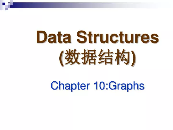
Data Structures ( 数据结构 ) C hapter 1 0 :Graphs. Vocabulary. Adjacency matrix 邻接矩阵 Adjacency list 邻接表 Minimum Spanning tree 最小派生树. Graph 图 Vertex 顶点 Edge 边 Arc 弧 Directed Graph 有向图 Undirected Graph 无向图 Adjacent Vertices 邻接点 Path 路径 Cycle 圈 Strongly connected 强连通

E N D
Vocabulary • Adjacency matrix 邻接矩阵 • Adjacency list 邻接表 • Minimum Spanning tree 最小派生树 Graph图 Vertex顶点 Edge 边 Arc弧 Directed Graph 有向图 Undirected Graph 无向图 Adjacent Vertices 邻接点 Path 路径 Cycle 圈 Strongly connected 强连通 Weekly connected 弱连通 Disjoint 未连通 depth-first traversal 深度优先遍历 Breadth-first traversal 广度优先遍历
Introduction to Graphs • Recall that a list is a collection of components in which • each component (except one, the first) has exactly 1 predecessor. • each component (except one, the last) has exactly 1 successor. • multiple successors • Unique predecessor Each node may have multiple successors as well as multiple predecessors Figure 7-1 A tree • Linear List • Tree • Graph
Definition of graph • A Graph is a collection of nodes, called vertices, and a collection of line segments, called edges (or arc), that connecting pairs of vertices. • In other words, a graph consists of two sets, a set of vertices and a set of lines.
Terminology • Graph may be eitherdirected orundirected: • Directed graph(Digraph) • Each line has adirection (arrow head)to its successor. • The lines in a directed graph are known as arcs • G = (V, E),V:aggregate of Vertices , E:aggregate of edges。<vi, vj> ≠ <vj, vi>。
Terminology • Graph may be eitherdirected orundirected: • Undirected graph • Each line has nodirection. • The lines in a undirected graph are known as edges • G = (V,E), V:aggreaget of Vertices , E:aggreage of edges .<vi, vj> = <vj, vi>。
Terminology • Path: • A path is a sequence of vertices in which each vertex is adjacent to the next one. • In the following figure, {A, B, C, E} is one path and {A, B, E, F} is another. • Both directed and undirected graphs have paths.
Terminology Cycle? • Cycle • A cycle is apath consisting of at least three vertices that starts and ends with the same vertex. • In the following subfigure (b), B, C, D, E, B is a cycle. In a digraph, a path can only follow the direction of the arcs In an undirected graph, a path can move in either direction along the edge
Terminology Connected Unconnected • Loop • A loop is a special case of a cycle in whicha single arc beings and ends with the same vertex. • Connected • Two vertices are said to be connected if there is a path between them. • A graph is said to be connected if there is a path from any vertex to any other vertex.
Terminology • Connected (directed graph) • Strongly connected • A directed graph is strongly connected if there is a path from each vertex to every other vertex in the digraph. • Weakly connected • A directed graph is weakly connected if at least two vertices are not connected. • Disjoint • A graph is disjoint if it is not connected.
Terminology • Degree • The degree of a vertex is the number of lines incident to it. • The degrees of the nodes A, C, D, F = 1 • The degrees of the nodes B, E = 3
Terminology • The degree of a vertex is thesum of the indegree and outdegree of lines incident to it. • The outdegree of a vertex in a digraph is the number of arcs leaving the vertex. • The indegree is the number of arcs entering the vertex.
Operations Add Vertex
Operations Delete Vertex Add edge
Operations Delete edge Find vertex
Traverse Graph • Traverse graph each vertex of the graphs be processed once and only once we must ensure that we process the data in each vertex only once. There are multiple paths to a vertex, we use a visited flag at each vertex to solve this problem. • Depth-first Traversal • Breadth-first Traversal
Depth-first Traversal Depth-first traversal of a tree We process all of a vertex’s descendents before we move to an adjacent vertex.
Depth-first Traversal • In the depth –first traversal all of a node’s descendents are processed before moving to an adjacent • depth-first traversal of a graph • processing the first vertex • Select any vertex adjacent to the first vertex and process it • Select an adjacent vertex until we reach a vertex with no adjacent entries, back out of the structure.(stack) The order in which the adjacent vertices are processed depends on how the graph is physically stored.
Depth-first Traversal We Begin by pushing the first vertex A into the stack We then loop, pop the stack, and , after processing the vertex. Push all of the adjacent vertices into the stack. Such as process Vertex X at step 2, we pop x from the stack process it, and then push the adjacent vertices G and H into the stack. When the stack is empty, the traversal is completes.
Breadth-first Traversal Breadth-first traversal of a tree We processing all adjacent vertices of a vertex before going to the next level
Breadth-first Traversal • In the Breadth –first traversal all adjacent vertices are processed before processing the descendents of a vertex. • Breadth-first traversal of a graph • processing the first vertex • Processing all of the first adjacent vertices • Pick the first adjacent vertex and processing all of its adjacent vertices, then the second adjacent vertex and so forth until we finished.(Queue)
Breadth-first Traversal We begin by enqueuing vertex A in the queue We the loop, dequeuing the queue and processing the vertex from the front of the queue. After processing the vertex, we place all of its adjacent vertices into the queue. When the queue is empty, the traversal is complete
Graph Storage Structure • Represent a graph we need to store two sets • The vertices of the graph • The edges or arcs of the graph • Two most common structures • Arrays • Linked list
Adjacency Matrix • One-dimensional array to store the vertices • Two-dimensional array to store the edges or arcs
Adjacency List • Two-dimensional linked list to store the edges or arcs
Graph Algorithms • Graph data Structure
Graph Algorithms • Create Graph • Insert Vertex • Delete Vertex • Insert Arc • Delete Arc • Retrieve Vertex • First Arc • Traverse
Depth-first Traversal Algorithm • 2 end if • Process vertex at stack top • 3 loop (not emptyStack(stack)) • 1 popStack(stack,vertexPtr) • 2 process(vertex->dataPtr) • 3 vertexPtr->processed =2 • Push all Vertices from adjacency list • 4 arcwalkPtr=vertexPr->arc • 5 loop( arcwalkPtr not null) • 1 vertToPtr=arcwalkPtr->destination • 2 if (vertToPtr->processed is 0) • 1 puchStack(sack,VertToPtr) • 2 vertToPtr->Processed =1 • 3 end if • 4 arcwalkPtr=arcwalkPtr->nextArc • 6 end loop • 4 end loop • 2 end if • 3 walkPtr-walkPtr->nextVertex • 8 end loop • 9 destroyStack(stack) • Return • End depthfirst Algorithm depthfirst (val graph<metadata> Processing the keys of the graph is depth-first order. Pre graph is a pointer to a graph head structure Post vertices “processed” • If (empty graph) • Return Set processed flags to not processed 2 walkPtr=graph.first • Loop (walkPtr) 1 walkPtr->processed = 0 2 walkPtr =walkPtr->nextVertex • End loop Process each vertex in list • createStack(stack) 6 walkPtr=graph.first 7 loop(walkPtr not null) 1 if (walkPtr->Processed <2) 1 if (walkPtr->processed <1) Push and set flag to stack 1 puchStack(stack,walker) 2 walkPtr->processed =1
Breadth-first Traversal Algorithm • Enqueue and set processed flag to 1 • 1 enqueue(queue,walkPtr) • 2 walkPtr->Processed =1 • 2 end if • How process descendents of vertex at queue first • 3 loop (not emptyQueue(queue)) • 1 dequeue(queue,vertexPtr) • Process Vertex and flag as processed • 2 process(vertexPtr) • 3 vertxPtr->processed =2 • Enqueue all vertices from adjacency list • 4 arcPtr=vertexPtr->arc • 5 loop (arcPtr not null) • 1 toPtr =arcPtr->destination 2 if (toPtr -> processed =1) 1 enqueue(queue,toPtr) • 2 toPtr->processed =1 • 3 end if • 4 arcPtr=arcPtr->nextArc • 6 end loop • 4 end loop • 2 end if • 3 walkPtr=walPtr->nextVertex • 9 end loop • 10 destroyQueue(queue) • 11 return • End breadthfirst Algorithm Breadthfirst (val graph<metadata> Processing the keys of the graph is Breadth-first order. Pre graph is a pointer to a graph head structure Post vertices “processed • If (empty graph) 1 return 2 End if Fist se all processed flags to not processed Falg:0– not processed, 1– enqueued, 2– processed • createqueue(queue) • walkPtr=graph.first • Loop (walkPtr not null) 1 walkPtr->processed =0 2 walkPtr=walkPtr->nextVertex • End loop Process each vertex in vertex list • walkPtr =graph.first • Loop (walkPtr not null) 1 if (walkPtr->Processed <2) 1 if (walkPtr->Processed <1)
Networks City airline Network • A network is a graph whose lines are weighted. It is also known as a weighted graph.
Minimum Spanning Tree • A spanning tree is a tree that contains all of the vertices in the graph • A minimum spanning tree of a network such that the sum of its weights are guaranteed to be minimal. if there are duplicate weights, then these may be one or more minimum spanning tree.
Minimum Spanning Tree City airline Network
Minimum Spanning Tree • From all the vertices in the tree. Select the edge with minimal value to a vertex not currently in the tree and insert it into the tree.
Shortest path • We find the shortest path between to vertices in network • The Dijkstra algorithm is used to find the shortest path between any two nodes in a graph Example : we need to find the shortest path from vertex A to any other vertex in the graph.
Shortest path • Insert the first vertex into the tree • From every vertex already in the tree , examine the total path length to all adjacent vertices not in the tree. Select the edge with the minimum total path weight and insert it into the tree • Repeat step 2 until all vertices are in the tree
Summary A graph is a collection of nodes, called vertices, and a collection of line segments connection pairs of nodes, called edges or arcs. Graphs may be directed or undirected. A directed graph, or digraph is a graph is which each line has s direction. An undirected graph is a graph in which there is no direction on the lines. A line in a directed graph is called an arc. In a graph, two vertices are said to be adjacent if an edge directly connects them A path is a sequence of vertices in which each vertex is adjacent to the next one A cycle is a path of at least three vertices that starts and ends with the same vertex A loop is a special case of a cycle is which a single arc begins with the same vertex
Summary • A graph is said to be connected if ,for any two vertices, there is a path from one to the other. A graph is disjointed if it is not connected. • The degree of a vertex is the number of the vertices adjacent to it. The outdegree of a vertex is the number of arcs leaving the node; the indegree of a vertex is the number of arcs entering the node. • Six operations have been defined for a graph:add a vertex, delete a vertex, add an edge, delete an edge, find a node, and traverse the graph. • There are two standard graph traversals: depth-first and breadth first. • In the depth-first traversal, all of the node’s descendents are processed before moving to an adjacent node • In the breadth-first traversal, all of the adjacent vertices are processed before processing the descendents of a vertex
Summary To represent a graph in a computer, we need to store two sets of information: the first sets represents the vertices and the second sets represents the edges. The most common methods used to store a graph are the adjacency matrix method and the adjacency list methods A network is a graph whose lines are weighted. A spanning tree is a graph whose lines are weighted A minimum spanning tree is a spanning tree in which the total weight of the edges is the minimum. Another common algorithm in a graph is to find the shotest pathe between two vertices.