Download
1 / 15
190 likes | 713 Views
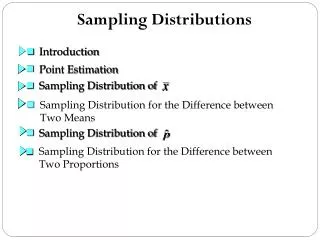
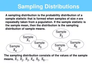
Sampling Distributions. A statistic is random in value … it changes from sample to sample. The probability distribution of a statistic is called a sampling distribution. The sampling distribution can be very useful for evaluating the reliability of inference based on the statistic.

E N D
Sampling Distributions • A statistic is random in value … it changes from sample to sample. • The probability distribution of a statistic is called a sampling distribution. • The sampling distribution can be very useful for evaluating the reliability of inference based on the statistic.
Central Limit Theorem (CLT) • If a random sample of sufficient size (n≥30) is taken from a population with mean m and variance s2>0, then • the sample mean will follow a normal distribution with mean m and variance s2/n,
CLT (continued) • the sum of the data will follow a normal distribution with mean nm and variance ns2. • The CLT can be used with any sample size if the underlying data follows a normal distribution.
Standardizing for the CLT • Z formulae for the CLT include:
Joint Probability Distributions • Many situations involve more than one random variable of interest. In these cases, a multivariate distribution can be used to describe the probability distributions of all random variables simultaneously.
Joint Probability Distributions for Discrete Random Variables • Joint Probability Mass Function (pmf) • Let X and Y be discrete random variables defined on the sample space S. The joint pmf, p( x, y ) is defined for each pair of ( x, y ) to be p( x, y ) = P( X=x, Y=y ) • Note: This is equivalent to P( X=x and Y=y )
Joint PMF • Properties of a Joint PMF • 0 ≤ p( x, y ) ≤ 1 • ∑x ∑y p( x, y ) = 1 • P( ( x, y ) A ) = ∑∑( x, y ) A p( x, y )
Marginal PMF • Let X and Y be discrete random variables with pmf p( x, y ) defined on the sample space S. The marginal pmf of X is pX(x) = ∑y p( x, y ) • Similarly, the marginal pmf of Y is pY(y) = ∑x p( x, y )
Independent Random Variables • Let X and Y be discrete random variables with pmf p( x, y ). • X and Y are independent if and only if p( x, y ) = px( x ) py( y ).
Extension of Joint PMF to Casewith n Discrete Random Variables • For n discrete random variables x1, x2,…, xn • the joint pmf is p( x1, x2,…, xn ) = P( X1=x1, X2=x2, …, Xn=xn ) • The marginal distribution for xk is p( x1, x2,…, xn ) = ∑x1 ∑x2…∑xk-1∑xk+1…∑xn p( x1, x2,…, xn )
Joint Probability Distributions for Continuous Random Variables • Joint Probability Distribution Function (pdf) • Let X and Y be continuous random variables defined on the sample space S. The joint pdf, f( x, y ) is a function such that: • f( x, y ) ≥0 • f( x, y ) dy dx = 1 • P( ( x, y ) A ) = ( x, y ) A f( x, y ) dy dx
Marginal PMF • Let X and Y be continuous random variables with pdf f( x, y ). The marginal pdf’s of X and Y are: fX(x) = y f( x, y ) dy • Similarly, the marginal pmf of Y is fy(y) = xf( x, y ) dx
Independent Random Variables • Let X and Y be continuous random variables with pdf f( x, y ). • X and Y are independent if and only if f( x, y ) = fx( x ) fy( y ).
Extension of Continuous PDF to Casewith n Continuous Random Variables • For n continuous random variables x1, x2, …, xn • the joint pdf f( x1, x2,…, xn ) has all the properties of a pdf • The marginal distribution for xk is f( x1, x2,…, xn ) = x1x2… xk-1 xk+1… xn f( x1, x2,…, xn )
Independent Random Variables • Let X and Y be continuous random variables with pdf f( x, y ). • X and Y are independent if and only if f( x, y ) = fx( x ) fy( y ). • X1, X2,…, Xn are mutually independent if and only if f( x1, x2,…, xn ) = f1(x1) f2(x2) … fn (xn)