Download
1 / 30
300 likes | 426 Views
Informed search methods Tuomas Sandholm Computer Science Department Carnegie Mellon University Read Section 3.5-3.7 of Russell and Norvig. Informed Search Methods. Heuristic = “to find”, “to discover”. “Heuristic” has many meanings in general How to come up with mathematical proofs

E N D
Informed search methodsTuomas SandholmComputer Science DepartmentCarnegie Mellon UniversityRead Section 3.5-3.7 of Russell and Norvig
Informed Search Methods Heuristic = “to find”, “to discover” • “Heuristic” has many meanings in general • How to come up with mathematical proofs • Opposite of algorithmic • Rules of thumb in expert systems • Improve average case performance, e.g. in CSPs • Algorithms that use low-order polynomial time (and come within a bound of the optimal solution) • % from optimum • % of cases • % PAC • h(n) that estimates the remaining cost from a state to a solution
Best-First Search f(n) function BEST-FIRST-SEARCH (problem, EVAL-FN) returns a solution sequence inputs: problem, a problem Eval-Fn, an evaluation function Queuing-Fn – a function that orders nodes by EVAL-FN return GENERAL-SEARCH (problem, Queuing-Fn) An implementation of best-first search using the general search algorithm. Usually, knowledge of the problem is incorporated in an evaluation function that describes the desirability of expanding the particular node. If we really knew the desirability, it would not be a search at all. “Seemingly best-first search”
Greedy Search function GREEDY-SEARCH (problem) returns a solution or failure return BEST-FIRST-SEARCH (problem, h) h(n) = estimated cost of the cheapest path from the state at node n to a goal state
Greedy Search… Not Optimal Incomplete O(bm) time O(bm) space Stages in a greedy search for Bucharest, using the straight-line distance to Bucharest as the heuristic function hSLD. Nodes are labeled with their h-values.
Beam Search • Use f(n) = h(n) but |nodes| K • Not complete • Not optimal
A* Search function A*-SEARCH (problem) returns a solution or failure return BEST-FIRST-SEARCH (problem, g+h) f(n) = estimated cost of the cheapest solution through n = g(n) + h(n)
f=291+380 =671 f=291+380 =671 A* Search… Stages in an A* search for Bucharest. Nodes are labeled with f = g+h. The h values are the straight-line distances to Bucharest.
A* Search… In a minimization problem, an admissible heuristic h(n) never overestimates the real value (In a maximization problem, h(n) is admissible if it never underestimates) Best-first search using f(n) = g(n) + h(n) and an admissible h(n) is known as A* search A* tree search is complete & optimal
Monotonicity of a heuristic h(n) is monotonic if, for every node n and every successor n’ of n generated by any action a, the estimated cost of reaching the goal from n is no greater than the step cost of getting to n’ plus the estimated cost of reaching the goal from n’: h(n) ≤ c(n,a,n’) +h(n’). This implies that f(n) (which equals g(n)+h(n)) never decreases along a path from the root. Monotonic heuristic => admissible heuristic. With a monotonic heuristic, we can interpret A* as searching through contours: Map of Romania showing contours at f = 380, f = 400 and f = 420, with Arad as the start state. Nodes inside a given contour have f-costs lower than the contour value.
Monotonicity of a heuristic… • A* expands all nodes n with f(n) < f*, and may expand some nodes right on the “goal contour” (f(n) = f*), before selecting a goal node. • With a monotonic heuristic, even A* graph search (i.e., search that deletes later-created duplicates) is optimal. • Another option, which requires only admissibility – not monotonicity – is to have the duplicate detector always keep the best (rather than the first) of the duplicates.
Completeness of A* • Because A* expands nodes in order of increasing f, it must eventually expand to reach a goal state. This is true unless there are infinitely many nodes with f(n) f* • How could this happen? • There is a node with an infinity branching factor • There is a path with finite path cost but an infinite number of nodes on it • So, A* is complete on graphs with a finite branching factor provided there is some positive constant s.t. every operator costs at least
Assumes h is admissible, but does not assume h is monotonic Proof of optimality of A* tree search Let G be an optimal goal state, and f(G) = f* = g(G). Let G2 be a suboptimal goal state, i.e. f(G2) = g(G2) > f*. Suppose for contradiction that A* has selected G2 from the queue. (This would terminate A* with a suboptimal solution) Let n be a node that is currently a leaf node on an optimal path to G. Situation at the point where a sub-optimal goal state G2 is about to be picked from the queue Because h is admissible, f* f(n). If n is not chosen for expansion over G2, we must have f(n) f(G2) So, f* f(G2). Because h(G2)=0, we have f* g(G2), contradiction.
Complexity of A* • Generally O(bd) time and space. • Sub-exponential growth when |h(n) - h*(n)| O(log h*(n)) • Unfortunately, for most practical heuristics, the error is at least proportional to the path cost
A* is optimally efficient A* is optimally efficient for any given h-function among algorithms that extend search paths from the root. I.e. no other optimal algorithm is guaranteed to expand fewer nodes (for a given search formulation) Intuition: any algorithm that does not expand all nodes in the contours between the root and the goal contour runs the risk of missing the optimal solution.
5 4 1 2 3 6 1 8 8 4 7 3 2 7 6 5 Heuristics (h(n)) for A* A typical instance of the 8-puzzle Start state Goal state Heuristics? h1: #tiles in wrong position h2: sum of Manhattan distances of the tiles from their goal positions h2 dominates h1: n, h2(n) h1(n)
Heuristics (h(n)) for A* … Comparison of the search costs and effective branching factors for the ITERATIVE-DEPENING-SEARCH and A* algorithms with h1, h2. Data are averaged over 100 instances of the 8-puzzle, for various solution lengths. It is always better to use a heuristic h(n) with higher values, as long as it does not overestimate. <= A* expands all nodes with f(n) < f*
Inventing heuristic functions h(n) Cost of exact solution to a relaxed problem is often a good heuristic for original problem. Relaxed problem(s) can be generated automatically from the problem description by dropping or relaxing constraints. Most common example in operations research: relaxing all integrality constraints and using linear programming to get an optimistic h-value. What if no dominant heuristic is found? h(n) = max [ h1(n), … hm(n) ] h(n) is still admissible & dominates the component heuristics Use probabilistic info from statistical experiments: “If h(n)=14, h*(n)=18”. Gives up optimality, but does less search Pick features & use machine learning to determine their contribution to h. Use full breath-first search as a heuristic? search time complexity of computing h(n)
Approximate A* versions (less search effort, but only an approximately optimal solution) • Dynamic weighting: f(n) = g(n) + h(n) +a [1- (depth(n) / N)] h(n) where N is (an upper bound on) depth of desired goal. Idea: Early on in the search do more focused search. Thrm: Solution is within factor (1+ a) of optimal. • Aa*: From open list, choose among nodes with f-value within a factor (1+ a) of the most promising f-value. Thrm: Solution is within factor (1+ a) of optimal Make the choice based on which of those nodes leads to lowest search effort to goal (sometimes picking a node with best h-value accomplishes this)
Best-bound search= A* search but uses tricks in practice • A* search was invented in the AI research community • Best-bound search is the same thing, and was independently invented in the operations research community • With heavy-to-compute heuristics such as LP, in practice, the commercial mixed integer programming solvers: • Use parent’s f value to queue nodes on the open list, and only evaluate nodes exactly when (if) they come off the open list • => first solution may not be optimal • => need to continue the search until all nodes on the open list look worse than the best solution found • Do diving. In practice there is usually not enough memory to store the LP data structures with every node. Instead, only one LP table is kept. Moving to a child or parent in the search tree is cheap because the LP data structures can be incrementally updated. Moving to another node in the tree can be more expensive. Therefore, when a child node is almost as promising as the most-promising (according to A*) node, the search is made to proceed to the child instead. • Again, need to continue the search until all nodes on the open list look worse than the best solution found
Iterative Deepening A* (IDA*) function IDA*(problem) returns a solution sequence inputs: problem, a problem static: f-limit, the current f-COST limit root, a node root MAKE-NODE(INITIAL-STATE[problem]) f-limit f-COST(root) loop do solution, f-limit DFS-CONTOUR(root,f-limit) ifsolution is non-null then returnsolution iff-limit = then return failure; end function DFS-CONTOUR(node,f-limit) returns a solution sequence and a new f-COST limit inputs: node, a node f-limit, the current f-COST limit static: next-f, the f-COST limit for the next contour, initially iff-COST[node] > f-limitthen return null, f-COST[node] if GOAL-TEST[problem](STATE[node]) then returnnode, f-limit for each node s in SUCCESSOR(node) do solution, new-f DFS-CONTOUR(s,f-limit) ifsolution is non-null then returnsolution, f-limit next-f MIN(next-f, new-f); end return null, next-f f-COST[node] = g[node] + h[node]
IDA* … Complete & optimal under same conditions as A*. Linear space. Same O( ) time complexity as A*. If #nodes grows exponentially, then asymptotically optimal space.
IDA* … • Effective e.g. in 8-puzzle where f typically only increases 2-3 times 2-3 iterations. • Last iteration ~ A* • Ineffective in e.g. TSP where f increases continuously • each new iteration only includes one new node. • If A* expands N nodes, IDA* expands O(N2) nodes • Fixed increment ~1/ iterations • Obtains -optimal solution if terminated once first solution is found • Obtains an optimal solution if search of the current contour is completed
A* vs. IDA* Map of Romania showing contours at f = 380, f = 400 and f = 420, with Arad as the start sate. Nodes inside a given contour have f-costs lower than the contour value.
Memory-bounded search algorithms }use too little memory • IDA* 1985 • Recursive best-first search 1991 • Memory-bounded A* (MA*) 1989 • Simple memory-bounded A* (SMA*) 1992 …
A 13(15) A A A 12 12 13 A G 0+12=12 13 10 8 B G B B G 10+5=15 8+5=13 15 18 H 15 13 10 10 8 16 C D H I A A A 20+5=25 16+2=18 15(15) 15(24) 20(24) 20+0=20 A 8 10 10 8 8 15 B B G E F J K 15 20() 24() 30+5=35 30+0=30 24+0=24 24+5=29 B G I D 15 24 C 25 24 20 Simple Memory-bounded A* (SMA*) (Example with 3-node memory) Progress of SMA*. Each node is labeled with its currentf-cost. Values in parentheses show the value of the best forgotten descendant. Search space f = g+h = goal 24+0=24 Optimal & complete if enough memory Can be made to signal when the best solution found might not be optimal - E.g. if J=19
SMA* pseudocode (from 1st edition of Russell & Norvig) Numerous details have been omitted in the interests of clarity function SMA*(problem) returns a solution sequence inputs: problem, a problem static: Queue, a queue of nodes ordered by f-cost Queue MAKE-QUEUE({MAKE-NODE(INITIAL-STATE[problem])}) loop do ifQueue is empty then return failure n deepest least-f-cost node in Queue if GOAL-TEST(n) then return success s NEXT-SUCCESSOR(n) if s is not a goal and is at maximum depth then f(s) else f(s) MAX(f(n),g(s)+h(s)) if all of n’s successors have been generated then update n’s f-cost and those of its ancestors if necessary if SUCCESSORS(n) all in memory then remove n from Queue if memory is full then delete shallowest, highest-f-cost node in Queue remove it from its parent’s successor list insert its parent on Queue if necessary insert s in Queue end