Download
1 / 26
260 likes | 293 Views
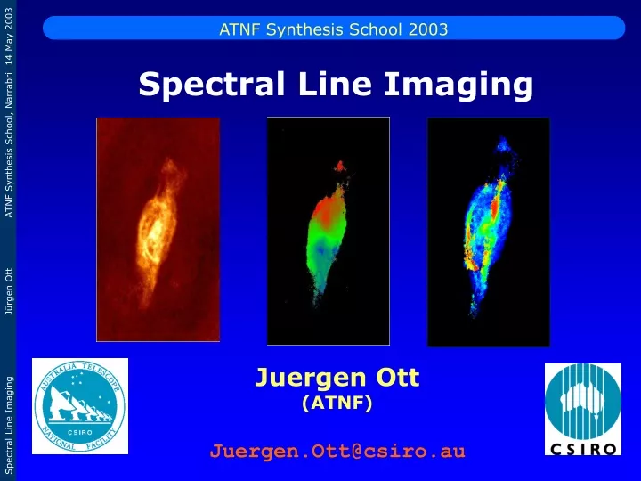
ATNF Synthesis School 2003. Spectral Line Imaging. Juergen Ott (ATNF). Juergen.Ott@csiro.au. Topics. Introduction to Spectral Lines Velocity Reference Frames Bandpass Calibration Continuum Subtraction Gibbs Phenomenon & Hanning Smoothing Data Cubes & Moment Maps. Literature:

E N D
ATNF Synthesis School 2003 Spectral Line Imaging Juergen Ott (ATNF) Juergen.Ott@csiro.au
Topics • Introduction to Spectral Lines • Velocity Reference Frames • Bandpass Calibration • Continuum Subtraction • Gibbs Phenomenon & Hanning Smoothing • Data Cubes & Moment Maps Literature: Synthesis Imaging in Radio Astronomy II, Chapters 11 & 12 Synthesis Imaging in Radio Astronomy, Chapter 17
Introduction to Spectral Lines What is a spectral line ? Origin: Light dispersion (prisma, slit) sharp intensity maxima on screen “extent in frequency much less than central frequency of feature” S (n, n0, A,Dn,t) atomic/molecular origin
Introduction to Spectral Lines Basic photon–matter interactions to produce spectral lines: Absorption (e.g., towards quasars) Spontaneous emission (e.g., HI, molecular lines, cascading recombination lines) Induced emission (Maser/Laser) Continuum: free-free, free-bound recombination (e.g., synchrotron emission, thermal bremsstrahlung) E hn
HI 21cm - - + + Introduction to Spectral Lines • Energy levels can be: • Atoms: electron orbits, • hyperfine states • (UV, optical, IR, radio) • Nuclei: excitations (shell model), g radiation • Solid states: bands (IR, opt), lattice modes (phonons) • Molecules: (electronic+) rotation, vibration, bending • (mm, submm, IR) CO (carbon monoxide) NH3 (ammonia)
Introduction to Spectral Lines • What can we learn from spectral lines? • Observables: frequency, shape (width), amplitude, (time) • Parameters of the Gas • (density, temperature, pressure, column density, …) • Parameters of the Environment • (radiation field, maser conditions, chemistry, magnetic field) • Kinematics • (expansion/contraction, infall/outflow, rotation curves, • galaxy clusters, turbulence, virialization theorem) • Distance (Hubble Law v=H r)
l – l0 l – l0 n0 – n vopt = c = c z = c vradio = c l0 l n0 vopt = vradio Velocity Reference Frames Relativistic Doppler Effect: n02 – n2 vradial = n02 + n2 approximations for vradial << c
Correlator Configurations • Correlator Configurations: • Bandwidth • Channel Separation (# Channels) • # Blocks (simultaneous observations of different frequencies) • # polarization products Cold molecular gas: linewidth ~ few km s-1 Rotation curves: Amplitude ~200 km s-1
FT x R(t) I(n) * Gibbs Phenomenon, Hanning Smoothing BUT… Ideal: Lag (cross-correlation) spectrum R(t) measured from - to But: Digital cross-correlation spectrometer Truncation of time lag spectrum R(t) Gibbs phenomenon or Gibbs ringing sinc (x) = sin(x) / x Nulls spaced by channel separation I(n) I’(n)
…etc 0.25 0.25 0.25 0.25 0.5 0.5 Gibbs Phenomenon, Hanning Smoothing Solution • Observe with more channels than necessary • Tapering sharp end of lag spectrum R() • Hanning smoothing: f()=0.5+0.5 cos (/T) • In frequency space: multiply channels with 0.25, 0.5, 0.25 half velocity resolution w/o Hanning w/ Hanning
~ ~ ~ Vij (n,t) = Gij (n,t) Vij (n,t) complex measured visibility Gain calibrated visibility Bij (n,t) bi (n,t) bj* (n,t) Bandpass Calibration Calibration: Bandpass baseline Bandpass antenna Gij (n,t) = G’ij (t) Bij (n,t) Measurement: Strong point source with flat (known) spectrum: Bandpass Calibrator, noise source @ source frequency & correlator setup, maybe several times Strong enough for high S/N per individual channel! Solve from N(N-1)/2 baselines for N antennas
Bandpass Calibration Perfect Bandpass Amplitude Frequency / Channel
Continuum Subtraction Data: continuum + spectral line emission (several sources with different sizes) Continuum subtraction uv plane image plane uvlin (MIRIAD tasks) contsub Visibilities Spectra Pixel (real & imaginary) • Additional flagging can be applied • Better continuum map • Allows shifting of reference center on string source, then back • no deconvolution which is non-linear
Continuum Subtraction • select line free channels • low order polynomial fit for each visibility (real & imaginary) • subtract fit from spectrum line only line + continuum Line free channels result of bandpass correction: flag it!
Data Cubes Data Cubes Declinationd Velocity v Channel Maps Right Ascensiona
Data Cubes Channel Maps Spectrum
Data Cubes Expanding Shell
Data Cubes position velocity
Data Cubes position – velocity cuts Major axis cut velocity position Minor axis cut Declination velocity velocity position Right ascension
mi := (x-a)i f(x) dx a := v f(v) dv - - Data Cubes – Moment Maps Moment maps Mathematical definition of central i-th moment (statistics): f(x): probability distribution a: center of mass of f(x)
M1 M2 M0 Data Cubes – Moment Maps Important Moments (as actually calculated, S over all spectral channels for each pixel): 0th moment: integrated intensity map [Jy km s-1] M0 = S I(v) Dv 1st moment: intensity weighted velocity map [km s-1] M1 = S I(v) v / S I(v) i=2, 2nd moment: 1s velocity dispersion [km s-1] M2 = S [I(v) (v-M1)2] / S I(v) Caution!!
Data Cubes – Moment Maps Moment 0 Moment 1 Moment 2
Conclusion Conclusion: Spectral line imaging is… powerful, versatile, fun!!!