Download

1 / 115
1.19k likes | 1.35k Views
Plant Reliability. Larry Jump JDSU Field Applications Engineer 814 692 4294 larry.jump@jdsu.com TAC 866 228 3762 Opt. 3 / 2. Agenda 3 major areas of concern. Coax Fiber Inside plant. Purpose. To provide better service to our customers in light of competition

E N D
Plant Reliability Larry Jump JDSU Field Applications Engineer 814 692 4294 larry.jump@jdsu.com TAC 866 228 3762 Opt. 3 / 2
Agenda 3 major areas of concern • Coax • Fiber • Inside plant
Purpose • To provide better service to our customers in light of competition • Maintain plant instead of reacting to problems • Be alerted to issues before the customer notices • Maintain reliability for essential services • To increase revenues
Internet not working Cracked hardline found with SWEEP Channel 12 video problems VOD not working WHY SWEEP? • Less manpower needed • Sweeping can does reduce the number of service calls
WHY SWEEP? Loose Face Plate No Termination
Sweep vs. Signal Level Meter Measurements • References:Sweep systems allow a reference to be stored eliminating the effect of headend level error or headend level drift. • Sweep Segments:Referenced sweep makes it possible to divide the HFC plant into network sections and test its performance against individual specifications. • Non-Invasive:Sweep systems can measure in unused frequencies. This is most important during construction and system overbuilding. • BEST Solution to align:Sweep systems are more accurate, faster and easier to interpret than measuring individual carriers.
Frequency Response Definition • System’s ability properly to transmit signals from headend to subscriber and back throughout the designed frequency range • Expected Results (Traditionally): n/10 + x = max flatness variation • where n = number of amplifiers in cascade • where x = best case flatness figure (supplied by manufacturer) • Expected Results in current HFC Networks: Typically < 3 to 4 dBmax flatness variation anywhere in the network (check with your Manager for max flatness variation limits)
Forward Path Considerations • Diverging System • Constant Outputs • Channel Plan to Match Fixed Signals • video / audio / digital carriers • Sweep Telemetry Carriers, 1MHz wide • System Noise • is the sum of cascaded amplifiers • Balance or Align (Sweep) • compensate for losses before the amp
Sweep Reference Considerations • Typically the node is used for the reference • Use test probe designed for node/amp • It’s a good engineering practice to store a new reference each day • Establish reference points to simplify ongoing maintenance (sweep file overlay) • Need to know amps hidden losses in return path (Block diagrams / Schematics) • Need to know where to inject sweep pulses and the recommended injection levels
H L Unity Gain in the forward path R R Each amplifier compensates for the loss in the cable and passives before the amplifier under test. The system is aligned so that the levels at each green arrow are exactly the same.
Why do we need Unity Gain? 32/26 30/24 31/25 29/23 22 22 22 22 23 23 23 If Unity Gain is not observed distortions and or noise build up quickly!
Forward Sweep Display Reference Name dB/div Max/Min Markers
A Sweep Finds Problems That Signal Level Measurements Miss Misalignment Standing Waves Roll off at band edges
Sweeping Reverse Path Goals • The objective in reverse path alignment is to maintain unity gain with constant inputs and minimize noise and ingress. • Set all optical receivers in the headend to same output level and ideally the same noise floor to optimize C/N ratio. • The reverse path noise is the summation of all noise from all the amplifiers in the reverse path. • Adjust sweep response to match 0dB flat line Sweep reference and 0dBmV Telemetry level
Before reverse sweeping begins…. • Optimize the upstream node • Splitting, combining and padding considerations in the headend.
Return Optics • We discuss this first because it has the greater impact on the MER at the CMTS input because it has the lowest dynamic range • Optimized by measuring NPR at the input to the CMTS by injecting different total power at the input to laser. • Carriers should be derated according to bandwidth using power per hertz. • Not part of the unity gain portion of the HFC plant. • Set up is laser and node specific
NPR Measurement • Measured by injecting a wideband noise source with a notch filter at the input. Then measuring essentially the noise to the notch at the output. • Measured as 10 log Power/hz of the signal/Power/hz of the notch noise • The lower the signal the lower the CNR, the higher the signal, the more distortion. • Input starts low and then raised in 1 dB steps
Power per Hertz Calculation Power per Hertz dBmV/Hz = Total Power – 10 Log (BW) dBmV/HZ = 45 – 10 Log (37,000,000) dBmV/ Hz = 45 – 10 (7.57) dBmV/ Hz = 45 – 75.7 dBmV/ Hz = -29.3 Total Power Input for 6.4 MHz 64 QAM dBmV = -29.3 + 10 Log (BW) dBmV = -29.3 + 10 Log (6,400,000) dBmV = -29.3 + 10 (6.8) dBmV = -29.3 + 68 dBmV = 38.7
Optical Receiver 20 dBmV NODE Optical Receiver NODE Optical Receiver NODE Optical Receiver NODE System Sweep Transmitter 3SR System Sweep Transmitter 3SR Stealth Sweep Stealth Sweep help FILE FREQ abc 2 def ghi 1 3 status jkl AUTO 4 5 mno 6 pqr CHAN alpha yz stu vwx 9 ENTER 7 8 SETUP x light . +/- space CLEAR FCN 0 PRINT SWEEP LEVEL SCAN TILT SPECT MOD C/N HUM REVERSE LEVEL 20 dBmV Reverse Combiner Pad for 0 dBmV All signal levels must be set to same output level at the optical receiver in the headend or hubsite with the same input at the node.
Optical Receiver 20 dBmV NODE 20 dBmV Optical Receiver NODE Optical Receiver NODE Optical Receiver NODE System Sweep Transmitter 3SR System Sweep Transmitter 3SR Stealth Sweep Stealth Sweep help FILE FREQ abc 2 def ghi 1 3 status jkl AUTO 4 5 mno 6 pqr CHAN alpha yz stu vwx 9 ENTER 7 8 SETUP x light . +/- space CLEAR FCN 0 PRINT SWEEP LEVEL SCAN TILT SPECT MOD C/N HUM REVERSE LEVEL 20 dBmV 20 dBmV Reverse Combiner Pad for 0 dBmV All signal levels must be set to same output level at the optical receiver in the headend or hubsite with the same input at the node.
Optical Receiver 20 dBmV NODE 20 dBmV Optical Receiver NODE 20 dBmV Optical Receiver NODE Optical Receiver NODE System Sweep Transmitter 3SR System Sweep Transmitter 3SR Stealth Sweep Stealth Sweep help FILE FREQ abc 2 def ghi 1 3 status jkl AUTO 4 5 mno 6 pqr CHAN alpha yz stu vwx 9 ENTER 7 8 SETUP x light . +/- space CLEAR FCN 0 PRINT SWEEP LEVEL SCAN TILT SPECT MOD C/N HUM REVERSE LEVEL 20 dBmV 20 dBmV Reverse Combiner 20 dBmV Pad for 0 dBmV All signal levels must be set to same output level at the optical receiver in the headend or hubsite with the same input at the node.
Optical Receiver 20 dBmV NODE 20 dBmV Optical Receiver NODE 20 dBmV Optical Receiver NODE 20 dBmV Optical Receiver NODE System Sweep Transmitter 3SR System Sweep Transmitter 3SR Stealth Sweep Stealth Sweep help FILE FREQ abc 2 def ghi 1 3 status jkl AUTO 4 5 mno 6 pqr CHAN alpha yz stu vwx 9 ENTER 7 8 SETUP x light . +/- space CLEAR FCN 0 PRINT SWEEP LEVEL SCAN TILT SPECT MOD C/N HUM REVERSE LEVEL 20 dBmV 20 dBmV Reverse Combiner 20 dBmV 20 dBmV Pad for 0 dBmV All signal levels must be set to same output level at the optical receiver in the headend or hubsite with the same input at the node.
Optical Receiver NODE Optical Receiver NODE Optical Receiver NODE Optical Receiver NODE System Sweep Transmitter 3SR System Sweep Transmitter 3SR Stealth Sweep Stealth Sweep help FILE FREQ abc 2 def ghi 1 3 status jkl AUTO 4 5 mno 6 pqr CHAN alpha yz stu vwx 9 ENTER 7 8 SETUP x light . +/- space CLEAR FCN 0 PRINT SWEEP LEVEL SCAN TILT SPECT MOD C/N HUM REVERSE NOISE Noise -35 dBmV Noise -35 dBmV Reverse Combiner Noise -35 dBmV Noise -35 dBmV Ideally all combined nodes should have same noise floor to maximize C/N ratio.
System Sweep Transmitter 3SR System Sweep Transmitter 3SR Stealth Sweep Stealth Sweep help FILE FREQ abc 2 def ghi 1 3 status jkl AUTO 4 5 mno 6 pqr CHAN alpha yz stu vwx 9 ENTER 7 8 SETUP x light . +/- space CLEAR FCN 0 PRINT SWEEP LEVEL SCAN TILT SPECT MOD C/N HUM Headend combining and splitting Other Return Services CMTS PathTrak Set top converter
Return Sweep considerations • Instead of point to multipoint, the system is multipoint to point • Unity gain at the inputs to the amplifiers • Telemetry carriers upstream and downstream • Noise and ingress are additive from the entire node. One bad drop can take down the entire node. • Channel Plan to match bursty digital signals. No sweep points on upstream carriers • Return Sweep compensates for losses after the amp • Set telemetry carrier level and sweep level to the same thing.
Advantages of return sweep over the older methods • Not as labor intensive as the older methods. • Align forward and reverse with the same stop at the amplifier • No cumbersome equipment in the field or the headend • Minimum use of bandwidth for test equipment • Control over the measurements • We are aligning the entire spectrum in both directions, not just 2 carriers!
5 things you need to know to set up your return path correctly • Know your equipment • Block diagrams of amplifiers, nodes, receivers, etc. • Test Equipment • Determine reverse sweep input levels • Determine reference points • Optimize return lasers portion first • Sweep coaxial portion of the plant
Port 4 Output Diplex TP Filter PORT 4 STATION H FWD FWD EQ PAD L REV Switch Port 5 Output Diplex TP Filter PORT 5 LOW PASS H FILTER L REV Switch Port 3 Port 6 Output Output Diplex Diplex TP TP Filter Filter PORT 3 PORT 6 H H L L REV REV Switch Switch Typical Node RF Block Diagram Fwd Signal from Optical Rcvr. Return Signal to Optical Transmitter
High Pass Filter STATION (1) IGC Plug-In EQ Aux EQ Plug-In EQ Interstage EQ PORT 1 Pre- Amplifier ALC PIN DIODE ATTEN Main Amplifier Bridger Amplifier Bridger Amplifier REVERSE RF TEST REV PAD Plug-In PAD Plug-In PAD REV PAD ALC Circuit Reverse Amplifier Low Pass Filter STATION (1) (1) Diplex Filter Diplex Filter Diplex Filter PORT 5 RF/AC Filter RF/AC Filter RF/AC Filter RF/AC Filter RF/AC Filter PORT 2 Plug-In EQ Plug-In PAD H L H L H L RF AC RF AC RF AC RF AC RF AC TRANSPONDER RF INTERFECE BRIDGE BRIDGER RF TEST AC Power AC Power AC Power AC Power AC Power PORT 3 PORT 6 (1) (1) (1) Test Points are Bi-Directional Notes: ALL test points can be -20 or -25dB Typical RF Bridging Amplifier Block Diagram
Know your test equipment Different test equipment operates differently. Size Matters!
H H H H L L L L How is a reference level determined? From trunk return 52 dBmvmax modem output 23db tap 2 dB drop loss 7 dB directional coupler 20dBmV at the reference point Does your system use this as the reference point? 23
H L Constant outputs in the return path? R R Return Equip. If the return amplifiers were balanced with constant outputs, the levels would vary widely by the time they got back to the headend. This is due to return amplifiers having several inputs.
The DSAM receives data from the transmitter and displays sweep from the headend unit 3. The field unit initiates the sweep through the return path at the reference level. 1. H L System Sweep Transmitter 3SR System Sweep Transmitter 3SR Stealth Sweep Stealth Sweep help FILE FREQ abc 2 def ghi 1 3 status The headend unit receives the sweep from the field unit, digitizes it’s own trace, and sends out on a forward telemetry pilot. jkl AUTO 4 5 mno 6 pqr CHAN alpha 2. yz stu vwx 9 ENTER 7 8 SETUP x light . +/- space CLEAR FCN 0 PRINT SWEEP LEVEL SCAN TILT SPECT MOD C/N HUM How does reverse sweep work? R R Return Equip. RF in RF out
H L System Sweep Transmitter 3SR System Sweep Transmitter 3SR Stealth Sweep Stealth Sweep help FILE FREQ abc 2 def ghi 1 3 status jkl AUTO 4 5 mno 6 pqr CHAN alpha Inject correct input sweep level Check for adjust raw sweep level Store reference file yz stu vwx 9 ENTER 7 8 SETUP x light . +/- space CLEAR FCN 0 PRINT SWEEP LEVEL SCAN TILT SPECT MOD C/N HUM Normalizing or Storing a Sweep Reference, reverse R R Return Equip. RF in RF out
H L System Sweep Transmitter 3SR System Sweep Transmitter 3SR Stealth Sweep Stealth Sweep help FILE FREQ abc 2 def ghi 1 3 status jkl AUTO 4 5 mno 6 pqr CHAN alpha Inject correct input sweep level Use the reverse sweep reference to compare and adjust amplifier output levels yz stu vwx 9 ENTER 7 8 SETUP x light . +/- space CLEAR FCN 0 PRINT SWEEP LEVEL SCAN TILT SPECT MOD C/N HUM Continuing On R R Return Equip. RF in RF out
Reverse Sweep Display Scale Factor Markers Start Frequency Stop Frequency Marker Frequencies Max Variation within Frequency Range Marker Relative Levels
Before After Loose Fiber Connector :A display an RF guy can understand • SC connector not pushed in all the way
Cross section of an Single Mode optical fiber Fiber Structure consists of a glass core, an outer protective glass cladding, and a buffer or coating Buffer Cladding Core 250 125 9 Side Front
Refraction Refraction is the bending of a ray of light at an interface. Cladding Core
IOR = Index of Refraction The Velocity of light in glass is different than the velocity of light in a vacuum. This ratio is known as the Index of Refraction. n = c / v n = refractive index c = velocity of light in a vacuum v = velocity of light in glass Glass Vacuum
Reflection Reflection is the abrupt change in the direction of a light ray at an interface. Cladding Core
Light in an optical fiber – Total Internal Reflection If, for a moment, we could magnify a fiber and slow down the speed of light, we could visualize one pulse as it reflects off the core/cladding boundary. This is known as Total Internal Reflection Core Magnified 25400x Timed slowed to 1 nanosecond Cladding
Microbending Macrobending Bending Large noticeable bends and microscopic irregularities can both attribute to loss in a fiber.
Common Connector Types SC Commonly referred to as Sam Charlie ST Commonly referred to as Sam Tom FC Commonly referred to as Frank Charlie LC Commonly referred to as Lima Charlie
Connector Configurations PC or UPS vs APC SC - PC SC - APC
Alignment Sleeve Alignment Sleeve Focused On the Connection Bulkhead Adapter Ferrule Fiber Fiber Connector Physical Contact Fiber connectors are widely known as the WEAKEST AND MOST PROBLEMATIC points in the fiber network.