Download
1 / 52
520 likes | 532 Views
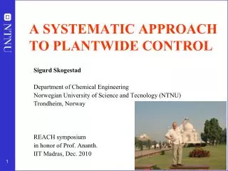
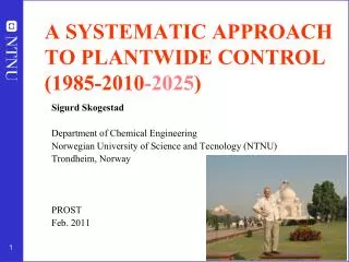
AN INTRODUCTION TO PLANTWIDE CONTROL. Sigurd Skogestad Department of Chemical Engineering Norwegian University of Science and Tecnology (NTNU) Trondheim, Norway Bratislava, jan. 2011. Arctic circle. North Sea. Trondheim. SWEDEN. NORWAY. Oslo. DENMARK. GERMANY. UK. NTNU, Trondheim.

E N D
AN INTRODUCTION TO PLANTWIDE CONTROL Sigurd Skogestad Department of Chemical Engineering Norwegian University of Science and Tecnology (NTNU) Trondheim, Norway Bratislava, jan. 2011
Arctic circle North Sea Trondheim SWEDEN NORWAY Oslo DENMARK GERMANY UK
NTNU, Trondheim
Plantwide control intro course: Contents • Overview of plantwide control • Step1-3. Selection of primary controlled variables based on economic : The link between the optimization (RTO) and the control (MPC; PID) layers- Degrees of freedom- Optimization- Self-optimizing control- Applications- Many examples • Step 4. Where to set the production rate and bottleneck • Step 5. Design of the regulatory control layer ("what more should we control") - stabilization - secondary controlled variables (measurements) - pairing with inputs - controllability analysis - cascade control and time scale separation. • Step 6. Design of supervisory control layer - Decentralized versus centralized (MPC) - Design of decentralized controllers: Sequential and independent design - Pairing and RGA-analysis • Summary and case studies
Dealing with complexity Main simplification: Hierarchical decomposition The controlled variables (CVs) interconnect the layers Process control OBJECTIVE Min J (economics); MV=y1s RTO cs = y1s Follow path (+ look after other variables) CV=y1 (+ u); MV=y2s MPC y2s Stabilize + avoid drift CV=y2; MV=u PID u (valves)
Main message • 1. Control for economics (Top-down steady-state arguments) • Primary controlled variables c = y1 : • Control active constraints • For remaining unconstrained degrees of freedom: Look for “self-optimizing” variables • 2. Control for stabilization (Bottom-up; regulatory PID control) • Secondary controlled variables y2 (“inner cascade loops”) • Control variables which otherwise may “drift” • Both cases: Control “sensitive” variables (with a large gain)!
Outline • Control structure design (plantwide control) • A procedure for control structure design I Top Down • Step 1: Define optimal operation • Step 2: Identify degrees of freedom and optimize for expected disturbances • Step 3: What to control ? (primary CV’s) (self-optimizing control) • Step 4: Where set the production rate? (Inventory control) II Bottom Up • Step 5: Regulatory control: What more to control (secondary CV’s) ? • Step 6: Supervisory control • Step 7: Real-time optimization
Practice: Tennessee Eastman challenge problem (Downs, 1991)(“PID control”)
How we design a control system for a complete chemical plant? • Where do we start? • What should we control? and why? • etc. • etc.
Alan Foss (“Critique of chemical process control theory”, AIChE Journal,1973): The central issue to be resolved ... is the determination of control system structure. Which variables should be measured, which inputs should be manipulated and which links should be made between the two sets? There is more than a suspicion that the work of a genius is needed here, for without it the control configuration problem will likely remain in a primitive, hazily stated and wholly unmanageable form. The gap is present indeed, but contrary to the views of many, it is the theoretician who must close it. • Carl Nett (1989): Minimize control system complexity subject to the achievement of accuracy specifications in the face of uncertainty.
Plantwide control = Control structure design • Not the tuning and behavior of each control loop, • But rather the control philosophy of the overall plant with emphasis on the structural decisions: • Selection of controlled variables (“outputs”) • Selection of manipulated variables (“inputs”) • Selection of (extra) measurements • Selection of control configuration (structure of overall controller that interconnects the controlled, manipulated and measured variables) • Selection of controller type (LQG, H-infinity, PID, decoupler, MPC etc.). • Previous work on plantwide control: • Page Buckley (1964) - Chapter on “Overall process control” (still industrial practice) • Greg Shinskey (1967) – process control systems • Alan Foss (1973) - control system structure • Bill Luyben et al. (1975- ) – case studies ; “snowball effect” • George Stephanopoulos and Manfred Morari (1980) – synthesis of control structures for chemical processes • Ruel Shinnar (1981- ) - “dominant variables” • Jim Downs (1991) - Tennessee Eastman challenge problem • Larsson and Skogestad (2000): Review of plantwide control
Control structure design procedure I Top Down • Step 1: Define operational objectives (optimal operation) • Cost function J (to be minimized) • Operational constraints • Step 2: Identify degrees of freedom (MVs) and optimize for expected disturbances • Step 3: Select primary controlled variables c=y1 (CVs) • Step 4: Where set the production rate? (Inventory control) II Bottom Up • Step 5: Regulatory / stabilizing control (PID layer) • What more to control (y2; local CVs)? • Pairing of inputs and outputs • Step 6: Supervisory control (MPC layer) • Step 7: Real-time optimization (Do we need it?) y1 y2 MVs Process
Step 1. Define optimal operation (economics) • What are we going to use our degrees of freedom u(MVs) for? • Define scalar cost function J(u,x,d) • u: degrees of freedom (usually steady-state) • d: disturbances • x: states (internal variables) Typical cost function: • Optimize operation with respect to u for given d (usually steady-state): minu J(u,x,d) subject to: Model equations: f(u,x,d) = 0 Operational constraints: g(u,x,d) < 0 J = cost feed + cost energy – value products
Control 3 active constraints 1 2 3 2 1 3 unconstrained degrees of freedom -> Find 3 CVs Step 2: Identify degrees of freedom and optimize for expected disturbances • Optimization: Identify regions of active constraints • Time consuming! 0
Step 3: Implementation of optimal operation • Optimal operation for given d*: minu J(u,x,d) subject to: Model equations: f(u,x,d) = 0 Operational constraints: g(u,x,d) < 0 → uopt(d*) Problem: Usally cannot keep uopt constant because disturbances d change How should we adjust the degrees of freedom (u)?
Implementation (in practice): Local feedback control! y “Self-optimizing control:” Constant setpoints for c gives acceptable loss d Local feedback: Control c (CV) Optimizing control Feedforward
Issue: What should we control? Question: What should we control (c)?(primary controlled variables y1=c) • Introductory example: Runner
Optimal operation - Runner Optimal operation of runner • Cost to be minimized, J=T • One degree of freedom (u=power) • What should we control?
Optimal operation - Runner Sprinter (100m) • 1. Optimal operation of Sprinter, J=T • Active constraint control: • Maximum speed (”no thinking required”)
Optimal operation - Runner Marathon (40 km) • 2. Optimal operation of Marathon runner, J=T • Unconstrained optimum! • Any ”self-optimizing” variable c (to control at constant setpoint)? • c1 = distance to leader of race • c2 = speed • c3 = heart rate • c4 = level of lactate in muscles
Optimal operation - Runner Conclusion Marathon runner select one measurement c = heart rate • Simple and robust implementation • Disturbances are indirectly handled by keeping a constant heart rate • May have infrequent adjustment of setpoint (heart rate)
Step 3. What should we control (c)? c = H y y – available measurements (including u’s) H – selection of combination matrix What should we control? Equivalently: What should H be? • Control active constraints! • Unconstrained variables: Control self-optimizing variables!
methanol + water valuable product methanol + max. 1% water cheap product (byproduct) water + max. 0.5% methanol Expected active constraints distillation 1. Valuable product: Purity spec. always active • Reason: Amount of valuable product (D or B) should always be maximized • Avoid product “give-away” (“Sell water as methanol”) • Also saves energy • Control implications valuable product: Control purity at spec. 2. “Cheap” product. May want to over-purify! Trade-off: • Yes, increased recovery of valuable product (less loss) • No, costs energy May give unconstrained optimum
c≥ cconstraint J Loss Back-off c 1. CONTROL ACTIVE CONSTRAINTS! • Active input constraints: Just set at MAX or MIN • Active output constraints: Need back-off • If constraint can be violated dynamically (only average matters) • Required Back-off = “bias” (steady-state measurement error for c) • If constraint cannot be violated dynamically (“hard constraint”) • Required Back-off = “bias” + maximum dynamic control error Jopt • Want tight control of hard output constraints to reduce the back-off • “Squeeze and shift”
Back-off = Lost production Time Example. Optimal operation = max. throughput. Want tight bottleneck control to reduce backoff! Rule for control of hard output constraints: “Squeeze and shift”! Reduce variance (“Squeeze”) and “shift” setpoint cs to reduce backoff
Unconstrained degrees of freedom Control “self-optimizing” variables 1. Old idea (Morari et al., 1980): “We want to find a function c of the process variables which when held constant, leads automatically to the optimal adjustments of the manipulated variables, and with it, the optimal operating conditions.” 2. “Self-optimizing control” = acceptable steady-state behavior (loss) with constant CVs. is similar to “Self-regulation” = acceptable dynamic behavior with constant MVs. 3. The ideal self-optimizing variable c is the gradient (c = J/ u = Ju) • Keep gradient at zero for all disturbances (c = Ju=0) • Problem: no measurement of gradient
Guidelines for selecting single measurements as CVs • Rule 1: The optimal value for CV (c=Hy) should be insensitive to disturbances d (minimizes effect of setpoint error) • Rule 2: c should be easy to measure and control (small implementation error n) • Rule 3: “Maximum gain rule”:c should be sensitive to changes in u (large gain |G| from u to c)orequivalently the optimum Jopt should be flat with respect to c (minimizes effect of implementation error n) Reference: S. Skogestad, “Plantwide control: The search for the self-optimizing control structure”, Journal of Process Control, 10, 487-507 (2000).
Optimal measurement combination • Candidate measurements (y): Include also inputs u H
No measurement noise (n=0) Nullspace method
With measurement noise cs = constant + u + + y K - + + c H Optimal measurement combination, c = Hy “=0” in nullspace method (no noise) “Minimize” in Maximum gain rule ( maximize S1 G Juu-1/2 , G=HGy) “Scaling” S1
Example: CO2 refrigeration cycle pH • J = Ws (work supplied) • DOF = u (valve opening, z) • Main disturbances: • d1 = TH • d2 = TCs (setpoint) • d3 = UAloss • What should we control?
CO2 refrigeration cycle Step 1. One (remaining) degree of freedom (u=z) Step 2. Objective function. J = Ws (compressor work) Step 3. Optimize operation for disturbances (d1=TC, d2=TH, d3=UA) • Optimum always unconstrained Step 4. Implementation of optimal operation • No good single measurements (all give large losses): • ph, Th, z, … • Nullspace method: Need to combine nu+nd=1+3=4 measurements to have zero disturbance loss • Simpler: Try combining two measurements. Exact local method: • c = h1 ph + h2 Th = ph + k Th; k = -8.53 bar/K • Nonlinear evaluation of loss: OK!
Refrigeration cycle: Proposed control structure Control c= “temperature-corrected high pressure”
Step 4. Where set production rate? • Where locale the TPM (throughput manipulator)? • Very important! • Determines structure of remaining inventory (level) control system • Set production rate at (dynamic) bottleneck • Link between Top-down and Bottom-up parts
TPM (Throughput manipulator) • TPM (Throughput manipulator) = ”Unused” degree of freedom that affects the throughput. • Definition (Aske and Skogestad, 2009). A TPM is a degree of freedom that affects the network flow and which is not directly or indirectly determined by the control of the individual units, including their inventory control. • Usually set by the operator (manual control), often the main feedrate
Production rate set at inlet :Inventory control in direction of flow* TPM * Required to get “local-consistent” inventory control
Production rate set at outlet:Inventory control opposite flow TPM
Step 5: Regulatory control layer Step 5. Choose structure of regulatory (stabilizing) layer (a) Identify “stabilizing” CV2s (levels, pressures, reactor temperature,one temperature in each column, etc.). In addition, active constraints (CV1) that require tight control (small backoff) may be assigned to the regulatory layer. (Comment: usually not necessary with tight control of unconstrained CVs because optimum is usually relatively flat) (b) Identify pairings (MVs to be used to control CV2), taking into account • Want “local consistency” for the inventory control • Want tight control of important active constraints • Avoid MVs that may saturate in the regulatory layer, because this would require either • reassigning the regulatory loop (complication penalty), or • requiring back-off for the MV variable (economic penalty) Preferably, the same regulatory layer should be used for all operating regions without the need for reassigning inputs or outputs.
Rules for pairing of variables and choice of control structure Main rule: “Pair close” • The response (from input to output) should be fast, large and in one direction. Avoid dead time and inverse responses! • The input (MV) should preferably effect only one output (to avoid interaction between the loops) • Try to avoid input saturation (valve fully open or closed) in “basic” control loops for level and pressure • The measurement of the output y should be fast and accurate. It should be located close to the input (MV) and to important disturbances. • Use extra measurements y’ and cascade control if this is not satisfied • The system should be simple • Avoid too many feedforward and cascade loops • “Obvious” loops (for example, for level and pressure) should be closed first before you spend to much time on deriving process matrices etc.
Example: Distillation • Primary controlled variable: y1 = c = xD, xB (compositions top, bottom) • BUT: Delay in measurement of x + unreliable • Regulatory control: For “stabilization” need control of (y2): • Liquid level condenser (MD) • Liquid level reboiler (MB) • Pressure (p) • Holdup of light component in column (temperature profile) Unstable (Integrating) + No steady-state effect Variations in p disturb other loops Almost unstable (integrating) Ts TC T-loop in bottom
Why simplified configurations?Why control layers?Why not one “big” multivariable controller? • Fundamental: Save on modelling effort • Other: • easy to understand • easy to tune and retune • insensitive to model uncertainty • possible to design for failure tolerance • fewer links • reduced computation load
y1 y2s K u2 G y2 Original DOF New DOF Degrees of freedom unchanged • No degrees of freedom lost by control of secondary (local) variables as setpoints become y2s replace inputs u2 as new degrees of freedom Cascade control:
”Advanced control” STEP 6. SUPERVISORY LAYER Objectives of supervisory layer: 1. Switch control structures (CV1) depending on operating region • Active constraints • self-optimizing variables 2. Perform “advanced” economic/coordination control tasks. • Control primary variables CV1 at setpoint using as degrees of freedom (MV): • Setpoints to the regulatory layer (CV2s) • ”unused” degrees of freedom (valves) • Keep an eye on stabilizing layer • Avoid saturation in stabilizing layer • Feedforward from disturbances • If helpful • Make use of extra inputs • Make use of extra measurements Implementation: • Alternative 1: Advanced control based on ”simple elements” • Alternative 2: MPC
Control configuration elements • Control configuration. The restrictions imposed on the overall controller by decomposing it into a set of local controllers (subcontrollers, units, elements, blocks) with predetermined links and with a possibly predetermined design sequence where subcontrollers are designed locally. Some control configuration elements: • Cascade controllers • Decentralized controllers • Feedforward elements • Decoupling elements • Selectors • Split-range control
Summary. Systematic procedure for plantwide control • Start “top-down” with economics: • Step 1: Identify degrees of freeedom • Step 2: Define operational objectives and optimize steady-state operation. • Step 3A: Identify active constraints = primary CVsc. Should be controlled to maximize profit) • Step 3B: For remaining unconstrained degrees of freedom: Select CV1s c based on self-optimizing control. • Step 4: Where to set the throughput (usually: feed) • Regulatory control I: Decide on how to move mass through the plant: • Step 5A: Propose “local-consistent” inventory (level) control structure. • Regulatory control II: “Bottom-up” stabilization of the plant • Step 5B:Control variables CV2 to stop “drift” (sensitive temperatures, pressures, ....) • Pair variables to avoid interaction and saturation • Finally: make link between “top-down” and “bottom up”. • Step 6: “Advanced control” system (MPC): • CVs: Active constraints and self-optimizing economic variables + look after variables in layer below (e.g., avoid saturation) • MVs: Setpoints to regulatory control layer. • Coordinates within units and possibly between units cs CV1 CV2