Download
1 / 35
350 likes | 482 Views
Quantum Lower Bounds You probably Haven’t Seen Before (which doesn’t imply that you don’t know OF them). Scott Aaronson, UC Berkeley 9/24/2002. QUANTUM ARGUMENTS. POLYNOMIALARGUMENTS. A History of Quantum Lower Bounds. A History of Quantum Lower Bounds. QUANTUM ARGUMENTS.

E N D
Quantum Lower Bounds You probably Haven’t Seen Before(which doesn’t imply that you don’t know OF them) Scott Aaronson, UC Berkeley 9/24/2002
QUANTUM ARGUMENTS POLYNOMIALARGUMENTS A History of Quantum Lower Bounds
A History of Quantum Lower Bounds QUANTUM ARGUMENTS BBBV’94: (n) lower bound for searching a list of n elements (i.e. Grover’s algorithm is optimal)
QUANTUM ARGUMENTS POLYNOMIALARGUMENTS A History of Quantum Lower Bounds BBCMW’98: bound for any symmetric Boolean function f(|X|) with f(k)f(k+1)
QUANTUM ARGUMENTS POLYNOMIALARGUMENTS A History of Quantum Lower Bounds Ambainis’00: (n) bounds for evaluating an AND-OR tree and for finding the ‘1’ in a permutation
QUANTUM ARGUMENTS POLYNOMIALARGUMENTS A History of Quantum Lower Bounds A’02: (n1/5) bound for the collision problem (deciding whether f:{1…n}{1…n} is 1-to-1 or 2-to-1) Shi’02: (n1/3) bound for collision with large range, (n2/3) for element distinctness
QUANTUM ARGUMENTS POLYNOMIALARGUMENTS A History of Quantum Lower Bounds Other results, including what I’ll talk about today
Truce Henceforth polynomial arguments shall be used for highly symmetric problems and for zero-error bounds, and quantum arguments otherwise. Whosoever disobeys, must post to quant-ph.
Talk Outline • Quantum Certificate Complexity • Recursive Fourier Sampling • Query Complexity & Quantum Gravity (special treat for Dave Bacon)
Background • f:{0,1}n{0,1} is a total Boolean function • D(f) (deterministic query complexity) • R0(f) (zero-error randomized) • R2(f) (bounded-error randomized) • Q2(f) (bounded-error quantum) Q0(f) (zero-error quantum) • QE(f) (exact quantum)
Certificate Complexity C(f) = maxX CX(f) • CX(f) = min # of queries needed to distinguish X from every Y s.t. f(Y)f(X) • Block Sensitivity bs(f) = maxX bsX(f) • bsX(f) = max # of disjoint blocks B{x1,…,xn} s.t. flipping B changes f(X) • Example: For f=MAJ(x1,x2,x3,x4,x5), letting X=11110, • 11110 11110 • CX(MAJ)=3 bsX(MAJ)=2 C(f) and bs(f)
Randomized Certificate Complexity RC(f) = maxX RCX(f) • RCX(f) = min # of randomized queries needed to distinguish X from any Y s.t. f(Y)f(X) with ½ prob. • Quantum Certificate Complexity QC(f) • Example: For f=MAJ(x1,…,xn), letting X=00…0, • RCX(MAJ) = 1 • Different notions of nondeterministic quantum query complexity: Watrous 2000, de Wolf 2002 RC(f) and QC(f)
Adversary Method(special case) Let D0,D1 be distributions over f-1(0), f-1(1) s.t. D0 looks “locally similar” to every 1-input, and D1 looks “locally similar” to every 0-input: Then
Claim: • Any randomized certificate for input X can be made nonadaptive • By minimax theorem, exists distribution over {Y:f(Y)f(X)} s.t. for all i, xiyi w.p. O(1/RC(f)) • Adversary method then yields • For upper bound, use “weighted Grover”
g g Example where C(f) = (QC(f)2.205)
New Quantum/Classical Relation For total f, where ndeg(f) = min degree of poly p s.t. p(X)0 f(X)=1 Previous: D(f)=O(Q2(f)2Q0(f)2) (de Wolf), D(f)=O(Q2(f)6) (Beals et al.)
Idea (follows Buhrman-de Wolf): Let p be s.t. p(X)0 f(X)=1 x1x2 – x2 + 2x3: x1x2, 2x3 are “maxonomials” Nisan-Smolensky: For every 0-input X and maxonomial M of p, X has a sensitive block whose variables are all in M Consequence: Randomized 0-certificate must intersect each maxonomial w.p. ½ Randomized algorithm: Keep querying a randomized 0-certificate, until either one no longer exists or p=0
Lemma: O(ndeg(f) log n) iterations suffice w.h.p. Proof: Let S be current set of monomials, and Initially (S) nndeg(f) ndeg(f)! We’re done when (S)=0 Claim: Each iteration decreases (S) by expected amount (S)/4e Reason: 1/e of (S) is concentrated on maxonomials, each of which decreases in degree w.p. ½
Fourier Sampling Given A:{0,1}n{0,1} Promise: A(x)=s·x(mod 2) for some s Return: g(s), for some known g:{0,1}n{0,1} (possibly partial) Classically: n queries needed Quantumly: 2 queries
g(s) x’s for which we can get s·x Recursive Fourier Sampling (RFS) g(s) x’s for which we can get s·x Fourier sampling composed log n times Classically: nlog n queries Quantumly: 2log n = n queries—or fewer?
Overview • Bernstein-Vazirani 1993: RFS puts BQP MA relative to oracle • Candidate for BQP PH • Could it put (say) BQP PH[polylog]? • Is uncomputing necessary? Why? • Goal: Show Q2(RFS) = (cd) for c>1 d = tree depth • Trouble: Suppose g(s) is a parity function Then Q2(RFSg) = 1
Plan of Attack • We define a nonparity coefficient of the function g,(g)[0,¾] • Measures how uncorrelated g is with parity of any subset of input bitsExamples: (Parity)=0, (Mod 3)=¾–O(1/n) • We then prove a lower bound: • If (g) is close to 0, this bound is useless. But we show that if (g)<0.146 then g is a parity function
The Nonparity Coefficient (g) Max * s.t. for some distributions D0 over g-1(0), D1 over g-1(1), for all z0n, t0g-1(0), t1g-1(1),
g(s) g(s) Theorem: Proof Idea: Uses Ambainis’ “most general” bound Let (x,y)R if xf-1(0), yf-1(1) “differ minimally” Weight inputs by D0,D1 from nonparity coefficient Then for all i and (x*,y*)R, RFS lower bound
Theorem: If • then (g)=0 (i.e. g is a parity function) • So either • the adversary method gives a good quantum lower bound, or • there exists an efficient classical algorithm “Pseudoparity” Functions Don’t Exist
OR AND AND OR AND OR OR OR x1 OR OR x2 AND x3 x4 In general, when can we do better for tree functions than by recursing on subtrees? (Saks-Wigderson, Santha) (Barnum-Saks: holds for any AND-OR tree) (Dürr-Høyer)
OR AND XOR OR AND XOR Does every Boolean function have a unique tree? Theorem (A’2000): Yes, modulo three “degeneracies” …
The Holographic Principle(‘t Hooft, Susskind, Bekenstein, Bousso…) A = surface area of 3D region(in Planck areas, 7.110-70 m2) N = # of bits it contains Tight for black holes
The Query Complexity Holographic Principle A = surface area of 3D region T = time needed to search it for a marked item (given finite speed of light)
Grover Search on a 2D Lattice n Quantum computer Marked item n
Can do in O(n3/4) time: searching a row classically takes n time; combining the results using Grover takes n1/4·n • In d dimensions, can do in O(n1/2+1/2d) • Implies “query complexity holographic principle”—when d=3, n1/2+1/6=n2/3 is O(A), in the case where A is minimized (a sphere) • Conjecture: n1/2+1/2d is optimal. Would imply “holographic” bound is tight for spheres (such as black holes…)