Download
1 / 59
590 likes | 663 Views
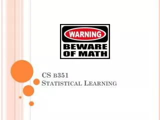
CS b351 Learning Probabilistic Models. Motivation. Past lectures have studied how to infer characteristics of a distribution, given a fully-specified Bayes net Next few lectures: where does the Bayes net come from ?. Win?. Strength. Opponent Strength. Win?. Opp. Def. Strength.

E N D
Motivation • Past lectures have studied how to infer characteristics of a distribution, given a fully-specified Bayes net • Next few lectures: where does the Bayes net come from?
Win? Strength Opponent Strength
Win? Opp. Def. Strength Offense strength Opp. Off. Strength Defense strength Score allowed Rush yds Rush yds allowed Pass yds
Opp injuries? Injuries? s At Home? Win? Opp. Def. Strength Offense strength Opp. Off. Strength Defense strength Score allowed Rush yds Rush yds allowed Pass yds Strength of schedule
Opp injuries? Injuries? s At Home? Win? Opp. Def. Strength Offense strength Opp. Off. Strength Defense strength Score allowed Rush yds Rush yds allowed Pass yds Strength of schedule
Agenda • Learning probability distributions from example data • Influence of structure on performance • Maximum likelihood estimation (MLE) • Bayesian estimation
Probabilistic Estimation problem • Our setting: • Given a set of examples drawn from the target distribution • Each example is complete (fully observable) • Goal: • Produce some representation of a belief state so we can perform inferences & draw certain predictions
Density Estimation • Given dataset D={d[1],…,d[M]} drawn from underlying distribution P* • Find a distribution that matches P* as “close” as possible • High-level issues: • Usually, not enough data to get an accurate picture of P*, which forces us to approximate. • Even if we did have P*, how do we define “closeness” (both theoretically and in practice)? • How do we maximize “closeness”?
What class of Probability Models? • For small discrete distributions, just use a tabular representation • Very efficient learning techniques • For large discrete distributions or continuous ones, the choice of probability model is crucial • Increasing complexity => • Can represent complex distributions more accurately • Need more data to learn well (risk of overfitting) • More expensive to learn and to perform inference
Two Learning problems • Parameter learning • What entries should be put into the model’s probability tables? • Structure learning • Which variables should be represented / transformed for inclusion in the model? • What direct / indirect relationships between variables should be modeled? • More “high level” problem • Once structure is chosen, a set of (unestimated) parameters emerge • These need to be estimated using parameter learning
Learning Coin Flips • Cherry and lime candies are in an opaque bag • Observe that c out of N draws are cherries (data)
Learning Coin Flips • Observe that c out of N draws are cherries (data) • Intuition: c/N might be a good hypothesis for the fraction of cherries in the bag(or it might not, depending on the draw!) • “Intuitive” parameter estimate: empirical distribution P(cherry) c / N(this will be justified more thoroughly later)
Structure Learning Example: Histogram bucket sizes • Histograms are used to estimate distributions of continuous or large #s of discrete values… but how fine?
Structure Learning: Independence Relationships • Compare table P(A,B,C,D) vs P(A)P(B)P(C)P(D) • Case 1: 15 free parameters (16 entries – sum to 1 constraint) • P(ABCD) = p1 • P(ABCD) = p2 • … • P(ABCD) = p15 • P(ABCD) = 1-p1-…-p15 • Case 2: 4 free parameters • P(A)=p1, P(A)=1-p1 • … • P(D)=p4, P(D)=1-p4
Structure Learning: Independence Relationships • Compare table P(A,B,C,D) vs P(A)P(B)P(C)P(D) • P(A,B,C,D) • Would be able to fit ALL relationships in the data • P(A)P(B)P(C)P(D) • Inherently does not have the capability to accurately model correlations like A~=B • Leads to biased estimates: overestimate or underestimate the true probabilities
Learned using independence assumption P(X)P(Y) Original joint distribution P(X,Y) Y X Y X
Structure Learning: Expressive Power • Making more independence assumptions always makes a probabilistic model less expressive • If the independence relationships assumed by structure model A are a superset of those in structure B, then B can express any probability distribution that A can X X X Y Z Y Z Y Z
C F1 F2 Fk Or F1 F2 Fk ? C
Arcs do not necessarily encode causality! A C B B C A 2 BN’s that can encode the same joint probability distribution
Reading off independence relationships • Given B, does the value of A affect the probability of C? • P(C|B,A) = P(C|B)? • No! • C parent’s (B) are given, and so it is independent of its non-descendents (A) • Independence is symmetric:C A | B => A C | B A B C
Learning in the face of Noisy Data • Ex: flip two independent coins • Dataset of 20 flips: 3 HH, 6 HT, 5 TH, 6 TT Model 1 Model 2 X Y X Y
Learning in the face of Noisy Data • Ex: flip two independent coins • Dataset of 20 flips: 3 HH, 6 HT, 5 TH, 6 TT Model 1 Model 2 X Y X Y Parameters estimated via empirical distribution (“Intuitive fit”) P(X=H) = 9/20 P(Y=H) = 8/20 P(X=H) = 9/20 P(Y=H|X=H) = 3/9 P(Y=H|X=T) = 5/11
Learning in the face of Noisy Data • Ex: flip two independent coins • Dataset of 20 flips: 3 HH, 6 HT, 5 TH, 6 TT Model 1 Model 2 X Y X Y Parameters estimated via empirical distribution (“Intuitive fit”) P(X=H) = 9/20 P(Y=H) = 8/20 P(X=H) = 9/20 P(Y=H|X=H) = 3/9 P(Y=H|X=T) = 5/11 Errors are likely to be larger!
Structure Learning: Fit vs complexity • Must trade off fit of data vs. complexity of model • Complex models • More parameters to learn • More expressive • More data fragmentation = greater sensitivity to noise
Structure Learning: Fit vs complexity • Must trade off fit of data vs. complexity of model • Complex models • More parameters to learn • More expressive • More data fragmentation = greater sensitivity to noise • Typical approaches explore multiple structures, while optimizing the trade off between fit and complexity • Need a way of measuring “complexity” (e.g., number of edges, number of parameters) and “fit”
Further Reading on Structure Learning • Structure learning with statistical independence testing • Score-based methods (e.g., Bayesian Information Criterion) • Bayesian methods with structure priors • Cross-validated model selection (more on this later)
Learning Coin Flips • Observe that c out of N draws are cherries (data) • Let the unknown fraction of cherries be q (hypothesis) • Probability of drawing a cherry is q • Assumption: draws are independent and identically distributed (i.i.d)
Learning Coin Flips • Probability of drawing a cherry is q • Assumption: draws are independent and identically distributed (i.i.d) • Probability of drawing 2 cherries is q*q • Probability of drawing 2 limes is (1-q)2 • Probability of drawing 1 cherry and 1 lime: q*(1-q)
Likelihood Function • Likelihood of data d={d1,…,dN} given q • P(d|q) = Pj P(dj|q) = qc (1-q)N-c i.i.d assumption Gather c cherry terms together, then N-c lime terms
Maximum Likelihood • Likelihood of data d={d1,…,dN} given q • P(d|q) = qc (1-q)N-c
Maximum Likelihood • Likelihood of data d={d1,…,dN} given q • P(d|q) = qc (1-q)N-c
Maximum Likelihood • Likelihood of data d={d1,…,dN} given q • P(d|q) = qc (1-q)N-c
Maximum Likelihood • Likelihood of data d={d1,…,dN} given q • P(d|q) = qc (1-q)N-c
Maximum Likelihood • Likelihood of data d={d1,…,dN} given q • P(d|q) = qc (1-q)N-c
Maximum Likelihood • Likelihood of data d={d1,…,dN} given q • P(d|q) = qc (1-q)N-c
Maximum Likelihood • Likelihood of data d={d1,…,dN} given q • P(d|q) = qc (1-q)N-c
Maximum Likelihood • Peaks of likelihood function seem to hover around the fraction of cherries… • Sharpness indicates some notion of certainty…
Maximum Likelihood • P(d|q) is the likelihood function • The quantity argmaxq P(d|q) is known as the maximum likelihood estimate (MLE)
Maximum Likelihood • l(q) = log P(d|q) = log [ qc(1-q)N-c]
Maximum Likelihood • l(q) = log P(d|q) = log [ qc(1-q)N-c]= log [ qc] + log [(1-q)N-c]
Maximum Likelihood • l(q) = log P(d|q) = log [ qc(1-q)N-c]= log [ qc] + log [(1-q)N-c]= c log q + (N-c) log (1-q)
Maximum Likelihood • l(q) = log P(d|q) = c log q + (N-c) log (1-q) • Setting dl/dq(q)= 0 gives the maximum likelihood estimate
Maximum Likelihood • dl/dq(q) = c/q– (N-c)/(1-q) • At MLE, c/q – (N-c)/(1-q) = 0=> q = c/N
Other MLE results • Categorical distributions (Non-binary discrete variables): take fraction of counts for each value (histogram) • Continuous Gaussian distributions • Mean = average data • Standard deviation = standard deviation of data
An Alternative approach: Bayesian Estimation • P(q|d) = 1/Z P(d|q) P(q) is the posterior • Distribution of hypotheses given the data • P(d|q) is the likelihood • P(q) is the hypothesis prior q d[1] d[2] d[M]
Assumption: Uniform prior, Bernoulli Distribution • Assume P(q) is uniform • P(q|d) = 1/Z P(d|q) = 1/Z qc(1-q)N-c • What’s P(Y|D)? qi Y d[1] d[2] d[M]
Assumption: Uniform prior, Bernoulli Distribution • Assume P(q) is uniform • P(q|d) = 1/Z P(d|q) = 1/Z qc(1-q)N-c • What’s P(Y|D)? qi Y d[1] d[2] d[M]
Assumption: Uniform prior, Bernoulli Distribution • =>Z = c! (N-c)! / (N+1)! • =>P(Y) = 1/Z (c+1)! (N-c)! / (N+2)! = (c+1) / (N+2) Can think of this as a “correction” using “virtual counts” qi Y d[1] d[2] d[M]