Lecture 2

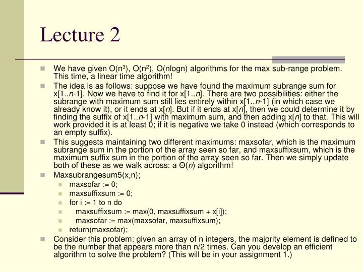
1. Lecture 2 • We have given O(n3), O(n2), O(nlogn) algorithms for the max sub-range problem. This time, a linear time algorithm! • The idea is as follows: suppose we have found the maximum subrange sum for x[1..n-1]. Now we have to find it for x[1..n]. There are two possibilities: either the subrange with maximum sum still lies entirely within x[1..n-1] (in which case we already know it), or it ends at x[n]. But if it ends at x[n], then we could determine it by finding the suffix of x[1..n-1] with maximum sum, and then adding x[n] to that. This will work provided it is at least 0; if it is negative we take 0 instead (which corresponds to an empty suffix). • This suggests maintaining two different maximums: maxsofar, which is the maximum subrange sum in the portion of the array seen so far, and maxsuffixsum, which is the maximum suffix sum in the portion of the array seen so far. Then we simply update both of these as we walk across: a Θ(n) algorithm! • Maxsubrangesum5(x,n); • maxsofar := 0; • maxsuffixsum := 0; • for i := 1 to n do • maxsuffixsum := max(0, maxsuffixsum + x[i]); • maxsofar := max(maxsofar, maxsuffixsum); • return(maxsofar); • Consider this problem: given an array of n integers, the majority element is defined to be the number that appears more than n/2 times. Can you develop an efficient algorithm to solve the problem? (This will be in your assignment 1.)

2. Time complexities of an algorithm • Worst-case time complexity of algorithm A T(n) = max|x|=n T(x) //T(x) is A’s time on x • Best-case … • Average-case time complexity of A T(n) = 1/2nΣ|x|=n T(x) assuming uniform distribution (and x binary). In general, given probability distribution P, the average case complexity of A is T(n) = Σ|x|=n P(x) T(x) • Space complexity defined similarly.

3. Asymptotic notations O,Ω,Θ,o • We say f(n) is O(g(n)) if there exist constants c > 0, n0 >0 s.t. f(n) ≤ cg(n) for all n ≥ n0. • We say f(n) is Ω(g(n)) if there exist constants c > 0, n0 >0 such that f(n) ≥ cg(n) for all n ≥ n0. • We say f(n) is Θ(g(n)) if there exist constants c1 > 0, c2 > 0, n0 >0 such that c1g(n) ≤ f(n) ≤ c2g(n) for all n ≥ n0. • We say f(n) is o(g(n)) if lim n → ∞f(n)/g(n) = 0. • We will only use asymptotic notation on non-negative valued functions in this course! • Examples: • n, n2, 3n2 + 4n + 5 are all O(n2), but n3 is not O(n2). • n2, (log n)n2, 4n2 + 5 are all Ω(n2), but n is not Ω(n2). • 2n2 + 3n + 4 is Θ(n2). • Exercise: What is the relationship between nlog (n) and e√n ? • Useful trick: If limn → ∞ f(n)/g(n) = c < ∞ for some constant c ≥ 0, then f(n) = O(g(n)). • We say an algorithm runs in polynomial time if there exists a k such that its worst-case time complexity T(n) is O(nk).

4. Average Case Analysis of Algorithms: • Let's go back to Insertion-Sort of Lecture 1. The worst-case running time is useless! For example, QuickSort does have Ω(n2) worst-case time complexity, we use it because its average-case running time is O(nlogn). In practice, we are usually only interested in the "average case". But what is the average case complexity of Insertion-Sort? • How are we going to get the average case complexity of an algorithm? Compute the time for all inputs of length n and then take the average? Usually hard! Alternatively, what if I give you one "typical" input, and tell you whatever the time the algorithm spends on this particular input is "typical" -- that is: it uses this much time on most other inputs too. Then all you need to do is to analyze the algorithm over this single input and that is the desired average case complexity!

5. Average-case analysis of Insertion-Sort Theorem. Average case complexity of Insertion-Sort is Θ(n2) . Proof. Fix a permutation π of integers 1,2,… , n such that (a) it takes at least nlogn – cn bits to encode π, for some constant c; and (b) since most permutations (> half) also require at least nlogn–cn bits to encode, π's time complexity is the average-case time complexity. • Now we analyze Insertion-Sort on input π. We encode π by the computation of Insertion-Sort: at j-th round of outer loop, assume the while-loop is executed for f(j) steps, thus the total running time on π is: T(π) = Σj=1..n f(j) (1) and, by Assignment 1 and (a), we can use Σj=1..n log f(j) ≥ nlogn -cn (2) bits to encode π. Subjecting to (1), when f(j)'s are all equal say = f0, the right side of (2) is maximized. Hence n log f0 ≥ Σj=1..n log f(j) ≥ nlogn - cn. Hence f0 ≥ n / 2c. Thus T(π) = Ω(n2). By (b), the average-case running time of Insertion-Sort is Ω(n2), hence we have Θ(n2), as the worst case is O(n2). 

6. 8 paradigms and 4 methods • In this course, we will discuss eight paradigms of algorithm design • reduce to known problem (e.g. sorting) • recursion • divide & conquer • invent (or augment) a data structure • greedy algorithm • dynamic programming • exploit problem structure (algebraic, geometric, etc.) • probabilistic or approximate solutions • And 4 methods of analyzing algorithms • counting -- usually for worst case • (probabilistic method -- for average case) • incompressibility method -- for average case • adversary arguments -- usually for worst case lower bounds

7. Paradigm 1. Reduce to known problem • In this method, you develop an algorithm for a problem by viewing it as a special case of a problem you already know how to solve efficiently. • Example 1: Decide if a list of n numbers contains repeated elements. • Solution 1: Using a double loop, compare each element to every other element. This uses Θ(n2) steps. • Solution 2: Sort the n numbers in O(nlogn) time, then find the repeated element in O(n) time. • Example 2: Given n points in the plain, find if there are three that are colinear. • Solution 1: For each triple of points, say P1 = (x1, y1), P2 = (x2, y2), P3 = (x3,y3), compute the slope of the line connecting P1 with P2 and P1 with P3. If they are the same, then P1, P2, P3 are colinear. This costs O(n3). • Solution 2: For each point P, compute the slopes of all lines formed by other points joined with P. If there is a duplicate element in this list, then there are three colinear points. Finding a duplicate among each list costs O(n log n), so the total cost is O(n2 log n). • For next lecture, read CLR, section 2.3 and chapter 4.