Download
1 / 56
560 likes | 564 Views
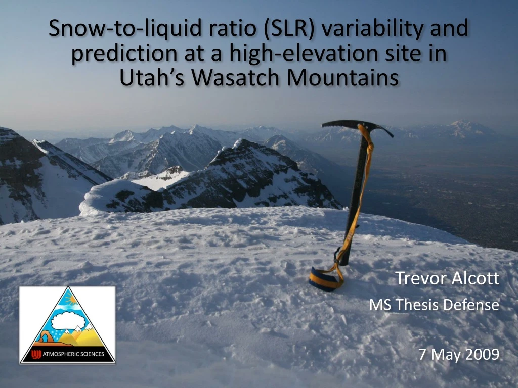
Snow-to-liquid ratio (SLR) variability and prediction at a high-elevation site in Utah’s Wasatch Mountains. Trevor Alcott MS Thesis Defense 7 May 2009. Outline. Why is snow-to-liquid ratio (SLR) important? What determines SLR? Datasets and Methodology SLR climatology at Alta

E N D
Snow-to-liquid ratio (SLR) variability and prediction at a high-elevation site in Utah’s Wasatch Mountains Trevor Alcott MS Thesis Defense 7 May 2009
Outline • Why is snow-to-liquid ratio (SLR) important? • What determines SLR? • Datasets and Methodology • SLR climatology at Alta • Relationship between meteorological conditions and SLR • Predicting SLR
What is snow-to-liquid ratio (SLR)? • SLR quantifies the amount of void space in snow • SLR = [new snow depth] / [new snow water equivalent (SWE)] • Other measures include snow density, water content, and specific gravity • snow density = ρwater / SLR • water content (%) = 100/SLR • specific gravity = 1/SLR (rarely used)
SLR vs. other measurements Low SLR High Density High SLR Low Density
Why is SLR important? • Interest in SLR originally stemmed from hydrological applications: if there are x inches of snow on the ground, what is the liquid equivalent? • Modern winter precipitation forecasting typically involves three steps: • 1. Quantitative precipitation forecast (QPF) • 2. Determination of precipitation type • 3. Application of SLR where precipitation type is snow: • Snowfall amount = QPF x SLR
Why is SLR important? • Snow clearing operations often based on specific snow amount thresholds, where perfect QPF is of limited value if an incorrect SLR is applied. • Avalanche forecasting- Casson (2008) relates SLR to snow shear strength • Accurate SLR and snowfall amount forecasts are critical for mountain communities like Alta, UT: • >1300 cm annual snowfall • 36 avalanche paths cross the only access road
The problem with SLR • Daily SLR varies considerably: • central Rocky Mountains- 3.9:1 to 100:1 • lowland sites across the US- 1.6:1 to 47:1 • What is the forecast snowfall amount for a QPF of 25 mm? 3:1 10:1 30:1 • Judson and Doesken (2000), Roebber et al. (2003)
What controls SLR? • Crystal type and size • Riming • Aggregation • Wind transport • Melting or sublimation aloft and at the surface • Rain on snow • Vapor pressure gradient-driven metamorphism and/or external compaction in high SWE events. (Settlement)
Crystal habit (shape) and SLR 25:1-100:1 15:1 20:1 12:1 12:1 10:1 10:1 10:1 Image: snowcrystals.com; SLR based on Power et. al. 1964, Dubé 2003, Cobb 2006
Riming and SLR 50:1 20:1 5:1 snowcrystals.com • Riming can decrease SLR by up to 90%. • most important for temperatures above −10°C; supercooled water more likely to be present • Fletcher (1962) defines riming rate:
Surface winds and SLR • Strong winds cause snow crystals to be dislodged and roll along the surface, removing outer features and decreasing SLR. • Snow transport begins at speeds of 8-10 m s-1. 15:1 4:1
Forecasting techniques: 10:1 “Rule” • “…assuming 10 inches of snow to 1 of water or some other factor, is subject to a large range of error because of the wide variability of this ratio for different kinds of snow.” -Report of the Chief Signal Officer, 1888 • “Looks like 0.1” of QPF for Salt Lake tonight. That’s an inch of snow, right?” -Jim Steenburgh, 2009
The 10:1 “Rule” • 10:1 is still used by: • RUC snowfall depth product • GFS and NAM MOS snowfall amount • snowfall forecasts at some NWS offices (other fixed ratios are also used) • Accuweather.com 15-day forecasts U.S. mean daily SLR (1971-2000) at NOAA Cooperative Observing sites (Baxter et al. 2005)
Improving on the 10:1 “Rule” • Despite known issues, 10:1 is still used by: • RUC snowfall depth product • Many NWS forecasters (or other fixed ratios) • Empirical techniques have been developed, relying on surface or in-cloud temperature • many of these techniques have not been verified • temperature typically explains just 25-40% of the variance, sometimes less than persistence (about 30%)
The SLR-Temperature Relationship R = 0.64 SLR 20:1 10:1 7:1 4:1 DENSITY 50 100 150 200 DENSITY 50 100 150 200 SLR 20:1 10:1 7:1 4:1 -25°C -20°C -15°C -10°C -5°C 0°C -15°C -10°C -5°C 0°C Surface temperature; Bossolasco 1954 700-hPa temperature (near surface); Lowry 1954
Forecasting Techniques: NWS Table • Although not intended for operational forecasting, the NWS new snowfall to estimated melt water conversion table relates SLR to surface temperature.
Forecasting Techniques: Neural Network • Roebber et al. (2003) used an ensemble of 10 artificial neural networks to forecast SLR in one of three classes: <9:1, 9:1 to 15:1, >15:1. 60% of forecasts were correct. • Neural networks are designed to resolve non-linear relationships between a series of inputs (e.g. mid-level temperature or humidity) and an output (SLR). PROCESSING ELEMENTS INPUTS OUTPUTS
Forecasting Techniques: Dubé Flowchart • Dubé (2003) used Power et al. (1964) and observations in Quebec to create a physically-based flowchart for predicting SLR and precipitation type. • Forecasts of SLR in one of 6 categories were correct for 83% of test cases.
Forecasting Techniques: UVV and T • Cobb and Waldstreichter (2005) combined vertical velocity with an SLR-temperature relationship. • UVV + ice saturation snow source layer • SLR(Tsource) weighted based on the depth of the source layer and the magnitude of UVV within it.
SLR Forecasting at the NWS • Most NWS offices use one or more of the following: • fixed ratio (often 10:1 or local climatology) • the NWS new snowfall to estimated melt water conversion table • the Cobb and Waldstreichter (2005) technique (WFO-SLC). 10:1 used where downward motion is forecast.
Cottonwood Canyons forecasts • Skill of NWS Cottonwood Canyons probabilistic snowfall forecasts has not improved over the past decade. • On average, snowfall verifies outside both forecast ranges 35% of the time.
Problems with existing approaches • NWS lookup table: overestimates SLR, problems with temperature inversions. • UVV and T: requires accurate forecasts of vertical velocity and relative humidity, ignores riming and wind. • 10:1 and other fixed ratios: large storm-to-storm variability • Much of SLR forecasting remains guesswork, with current tools often problematic, unverified and underutilized.
…the current operational practice of forecasting snow density, and hence snowfall depth, is still largely a nonscientific endeavor. -Roebber et. al. (2003)
A Different Approach • Past studies use data from multiple sites to study relationships between SLR and meteorological conditions and develop forecast algorithms. • Instead we use a single site with high quality of measurement and a high frequency of snow storms, and apply a straightforward regression technique to better understand SLR variability and improve SLR prediction.
Research Goals • Develop an SLR climatology for Alta, UT • Determine relationships between SLR and meteorological conditions at the study site. • Evaluate the use of stepwise multiple linear regression for SLR diagnosis and prediction.
Alta-Collins Snow Study Site Alta Google Earth view facing south Idaho Wyo. Nevada Utah Great Salt Lake Wasatch Mtns. KSLC Salt Lake Valley LCC CLN 1250 2250 3250 m • Collins (CLN) is located at Alta Ski Resort, on the south side of Little Cottonwood Canyon, at 2945 m (9660 ft) elevation.
Alta-Collins Snow Study Site Measurement site facing northeast • consistent and accurate measurements by snow safety professionals. • high frequency of snow storms (18 storms/y with 25 cm or more snowfall). • low frequency of mixed precipitation events during winter.
Data Description • Full CLN record covers 1980-2007, restricted to Nov-Apr 1999-2007 when hourly precipitation data are available. • 24-h (1200-1200 UTC) snow depth and SWE • Upper air data: North American Regional Reanalysis (NARR), every 3 h, for the grid point nearest to CLN. • Temperatures/wind/relative humidity during an event are the average of only 3-h periods where ≥ 0.25 mm SWE was recorded at CLN. • After quality control, the dataset contains 457 events.
Sources of Error and Quality Control • Undercatch: shielded and properly sited gauge. • Rain on snow: eliminate events where 650-hPa temperatures exceed 0°C, following Bourgouin (2000) • Other precipitation types: sleet is rare, FZDZ is light • Measurement/rounding errors: restrict to ≥ 5 cm snow and ≥ 2.8 mm SWE, following Judson and Doesken (2000), Roebber et al. (2003,2007) and Baxter et al. (2005). • Other sources not accounted for: • melting by Spring sun when T<0°C • settlement when snow ends well before measurement • measurement time not exactly 1200 UTC (maximum +/- 2 h)
3. Results Part A: Climatology
Distribution of SLR at Alta • Mean: 14.4:1 • (KSLC: 14.8:1) • Median: 13.3:1 • Mode: 10:1-12:1 • Max: 35.7:1 • Min: 3.6:1
“Wild Snow” • Wild snow, defined by Judson and Doesken (2000) as SLR ≥ 25:1, occurs in 5.7% of events, compared to 8% in the CO Park Range • SLR in wild snow events greatly exceeds the climatological 14.4:1 at Alta, which can lead to forecast busts. • NWS treatment of 20 mm QPF in 24h: • 14.4:1 - snow advisory • 30:1 - heavy snow warning • What conditions favor wild snow?
SLR by Month • Median SLR nearly constant in winter, highest in Mar, lowest in Apr. • Variability in SLR greatest in Feb, lowest during Apr. • 24 of the 26 wild snow events occur Dec-Feb. NOV DEC JAN FEB MAR APR
3. Results Part B: SLR and meteorological conditions
Vertical Profiles of R All 457 events 80 high SWE (>25 mm) events -0.76 -0.64 • typical elevation of the 650 hPa level is 3400 m (11000 ft) • Correlation coefficients are significant at the 99% level when |R|≥ 0.13 for all events and |R| ≥ 0.29 for high SWE events.
SLR and Temperature at Alta • SLR increases (decreases) with increasing temperature below (above) −15°C. • Wild snow occurs almost exclusively with temperatures between −12° and −18°C, the “dendritic growth zone” • Warm temperatures associated with a narrow range of SLR
SLR and Temperature at Alta • SLR is best related to the temperature of the primary snow growth region (Kyle and Wesley 1997) • high elevation mountain sites are close to the primary snow growth region (Wetzel et al. 2004) • high SLR near −15°C • dendrites form, crystal growth rate maximized • lower SLR below −15°C • plates/columns, slower growth rate • lower SLR above −15°C • plates/columns/needles • riming is more likely
SLR and wind speed at Alta • wide range of SLR occurs near 10 m s-1 • higher wind speeds associated with lower SLR and a smaller range • wild snow occurs only with speeds between 7 and 12 m s-1
SLR and SWE at Alta • Higher SWE is weakly related to lower SLR (R = −0.32) • Hyperbolas are a rounding artifact, represent equal snow depth • Wild snow occurs only for SWE less than 20 mm
SLR and SWE at Alta • compaction/increased settlement rate from overlying weight? • higher SWE events are also associated with: • warmer temperatures • higher wind speeds
3. Results Part C: Stepwise multiple linear regression
SMLR Procedure • 92 predictors: • CLN: SWE and surface temperature • NARR: temperature, wind speed/direction, RH • Square, cube, and inverse of predictors included to account for some non-linearity • Matlab Stepwise program proceeds in steps until reaching a local minimum in root-mean-square error of the fit: • add the most significant term (entrance tolerance 0.05) • remove the least significant term (exit tolerance 0.10)
Regression ResultsAll predictors All 457 events 80 high SWE (>25 mm) events • 13 predictors explain 68% of the variance in SLR for all events. • Approach is more effective for high SWE events; 88% of the variance explained by 9 predictors.
Comparison with Past Studies R2 (Observed vs. Regression Estimate) Alta High SWE Alta All
Regression ResultsTemperature and Wind All 457 events 80 high SWE (>25 mm) events • Reducing the field of predictors to temperature and wind only slightly reduces R2 for all events and the high SWE subset.
SLR Prediction • Regression using NARR data is a “perfect prog” technique and not a true test of forecast skill. • Biases in the NARR differ from those in forecast models. • Next step: run SMLR on a dependent set of archived model data, test the equation by making hindcasts for an independent set • Model data: 6-hourly, 12-36h NAM forecasts at 40-km resolution, dependent and independent sets of 177 and 179 events, respectively.
SLR Prediction • NAM SMLR approach shows some skill in forecasting SLR using only temperature and wind predictors. • SMLR performs better for 37 high SWE events (not shown), where R2 = 0.73 between forecast and observed. • Due to reduced sample size, results are somewhat sensitive to the choice of events in the independent and dependent sets.
Comparison of Forecast Techniques • SMLR offers an improvement over the use of fixed climatological or 10:1 ratios. • The NWS Table suffers from a high bias, and shows poor predictive ability. RMSE (Observed vs. Forecast)