Download
1 / 25
310 likes | 493 Views
Numerical Summary measures. Ch 3, Principle of Biostatistics Pagano & Gauvreau Prepared by Yu-Fen Li. Numerical Summary measures. Tables and graphs are extremely useful for organizing, visually summarizing , and displaying data.

E N D
Numerical Summary measures Ch 3, Principle of Biostatistics Pagano & Gauvreau Prepared by Yu-Fen Li
Numerical Summary measures • Tables and graphs are extremely useful for organizing, visually summarizing, and displaying data. • In order to make concise and quantitative statements, we rely on numerical summary measures. • We have various types of descriptive statistics which can provide a great deal of information about a set of observations.
Population vs. SampleParameter vs. Statistic • Population • A collection of subjects or events that share a common characteristic. • Sample • A portion of the population • Parameter • A description of some characteristic of a population. • Is fixed or constant & symbolized with Greek letters. • Statistic • A description of some characteristic of a sample. • May vary & typically symbolized with English letters.
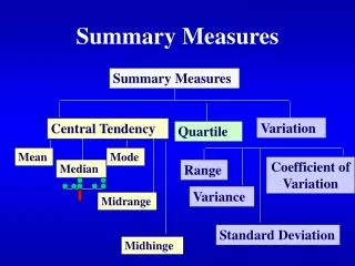
Numerical Summary measures • Measures of Central Tendency • Measures of Dispersion
Measures of Central Tendency • The most commonly investigated characteristic of a set of data is its center, or the point about which the observations tend to cluster. • There are three commonly used measures of central tendency: 1) mean, 2) median, and 3) mode.
Measures of Central Tendency –1. mean • Mean (arithmetic mean or average) is the most frequently used measure of central tendency. • Let Xi (x)ibe the observation of subject i, where i= 1, · · · , N(n). • The mean of the N(n) observations, represented by (), is defined as sample population
Measures of Central Tendency –1. mean • The mean can be used as a summary measure for both discrete and continuous measurements. • However, it is not appropriate for either nominal or ordinal data, except dichotomous data with values 0 and 1 • The mean of dichotomous data is the proportion of observations with a value of 1. • The method by which the mean is calculated takes into accounts the magnitude of every observation in a set of data, so the mean is extremely sensitive to unusual values
Measures of Central Tendency –2. median • The median is one measure of central tendency that is less sensitive to the value of each measurement. • The median is defined as the 50th percentile of a set of data, and it can be used as a summary measure for ordinal, discrete, and continuous data.
Measures of Central Tendency –2. median • Let xibe the observation of subject i, where i= 1, · · · , n. • Rank the observations from the smallest to the largest, and denote them as x(i), where i= 1, · · · , n. • If n is odd, the median is the middle value, i.e. • 10,20,30,40,50 : the median is 30 • If n is even, the median is the average of the two middlemost values, i.e. • 10,20,30,40 : the median is 25
Measures of Central Tendency –3. mode • A third measure of central tendency is the mode which can be used as a summary measure for all types of data. • The mode of a set of values is the observation that occurs most often. • When no number occurs more than once in a data set, there is no mode, e.g. 1,2,3,4,5,6 • There are possible multiple modes in a data set, e.g. 1,1,2,3,3
Measures of Dispersion • Range • Interquartile Range (IQR) • Variance and Standard Deviation • Coefficient of Variation
Measures of Dispersion –1. range • The range of a data set is defined as the difference between the largest observation (i.e. maximum) and the smallest (i.e. minimum). • The range is very easy to compute • The range is highly sensitive to extreme measurements
Measures of Dispersion –2. interquartile range • A second measure of variability is the interquartile range (IQR), calculated by subtracting the 25th percentile (Q1) of the data from the 75th percentile (Q3), • i.e. IQR = Q3 - Q1 • How to find the kth percentile of a set of data by hand? • We begin by ranking the n measurements from smallest to largest. • If nk/100 is an integer, the kth percentile of the data is the average of the (nk/100)th and (nk/100 +1)th largest observations. • If nk/100 is not an integer, the kth percentile is the (j+1)th largest measurement, where j is the largest integer that is less than nk/100
How to find the kthpercentile? • If nk/100 is an integer, the kth percentile of the data is the average of the (nk/100)th and (nk/100 +1)th largest observations. • n=12, 12*25%=3, 12*50%=6, 12*75%=9 • If nk/100 is not an integer, the kth percentile is the (j+1)th largest measurement, where j is the largest integer that is less than nk/100 • n=11, 11*25%=2.75, 11*50%=5.5, 11*75%=8.25 Q1 Q2 Q3 Q3 Q1 Q2
Percentiles • There is no standard definition of percentile; however all definitions yield similar results when the number of observations is very large • Nearest rank is often given in texts • Alternative methods include • Linear interpolation between closest ranks • Weighted percentile • Others • National Institute of Standards and Technology
Measures of Dispersion –3. variance and standard deviation • The variance is another commonly used measure of dispersion for a set of data • The ‘standard deviation’ (denoted as SD or s) of a set of data is the positive square root of the variance population sample
Measures of Dispersion –4. coefficient of variation • Because the SD has units of measurement, it is meaningless to compare SDs for two unrelated quantities • e.g. 5 cm vs. 5 kg • The coefficient of variation (CV) is defined as • the CV is a dimensionless number, so one can compare the CVs of two or more sets of data with different units.
Graph – Box(-and-Whisker) plots • A box plot is a convenient way of graphically depicting groups of numerical data through their quartiles. 1.5*IQR 1.5*IQR
What do we need for a box plot? • For the box: Q1, Q2, Q3 • For the whiskers: the adjacent values • the most extreme observations in the data set that are not more than 1.5 times the height of the box (i.e. 1.5 × IQR) beyond either quartile. • Therefore, they are not necessary to be the maximum and minimum in the data set
extreme values Upper Outer Fence outliers Upper Inner Fence upper adjacent value mean lower adjacent value Lower Inner Fence Lower Outer Fence
Empirical rule • When the data are symmetric and unimodel, we can say that • approximately 68% of the observations lie in the interval ± 1s (±1) , • about 95% in the interval ± 2s (±2), and • almost all the observations in the interval ± 3s (±3) • This is known as the 68–95–99.7 rule or the three-sigma rule.
Standard Normal Curve • P(−1 ≤ Z ≤ 1) = 0.682 • We will see the empirical rule again in Chapter 7 of the textbook.
Chebychev’s Inequality • When the data are not symmetric and unimodel, we cannot apply the empirical rule. • Chebychev’sinequality is less specific than the empirical rule, but it is true for any set of observations, no matter what its shape • For k=2,at least 75% of the data in the interval ± 2
Useful tools • R資料分析暨導引系統(R Data Analysis & Guiding System, RDAGS) • http://www.r-web.com.tw/ • free • no programming needed • Chinese version only (for now)