Download
1 / 90
900 likes | 1k Views
Explore scheduling in distributed systems to optimize processor utilization and process completion time. Understand system performance models and consider speedup factors for efficient processing. Learn about static and dynamic scheduling strategies for enhanced system performance.

E N D
The primary objective of scheduling is to enhance overall system performance metrics such as process completion time and processor utilization. The existence of multiple processing nodes in distributed systems present a challenging problem for scheduling processes onto processors and vice versa.
A system performance model • Depicts the relationship among algorithm, scheduling and architecture to describe the Inter process communication • Basically three types of model are there: • Precedence process model(DAG) Directed edges represent the precedence relationship
Communication process model • In this model processes co-exist and Communicate asynchronously. • Edges in this model represent the need of communication between the processes
Disjoint process model: • In this processes run independently and completed in finite time. • Processes are mapped to the processors to maximize the utilization of processesorsand minimize the turnaround time of the processes.
Partitioning a task into multiple processes for execution can result in a speedup of the total task completion time. The speedup factor S is a function S = F(Algorithm; System; Schedule)
S can be written as: Where OSPT = optimal sequential processing time CPT = concurrent processing time OCPTideal = optimal concurrent processing time Si = the ideal speedup by using multiple processor system over best sequential time Sd = the degradation of the system due to actual implementation compared to an ideal system
and n is the number of processors. The term is is the total computation of the concurrent algorithm where m is the number of tasks in the algorithm. Sd can be rewritten as: where
RP is Relative Processing: how much loss of speedup is due to the substitution of the best sequential algorithm by an algorithm better adapted for concurrent implementation. • RC is the Relative Concurrency which measures how far from optimal the usage of the n-processor is. It reflects how well adapted the given problem and its algorithm are to the ideal n-processor system. • The final expression for speedup S is
The term is called efficiency loss. It is a function of scheduling and the system architecture. It would be decomposed into two independent terms but this is not easy to do since scheduling and the architecture are interdependent. The best possible schedule on a given system hides the communication overhead (overlapping with other computations).
The unified speedup model integrates three major components • algorithm development • system architecture • scheduling policy
with the objective of minimizing the total completion time (makespan) of a set of interacting processes. If processes are not constrained by precedence relations and are free to be redistributed or moved around among processors in the system, performance can be further improved by sharing the workload • statically - load sharing • dynamically - load balancing
Speed up N- Number of processes - Efficiency Loss when implemented on a real machine. RC-relative concurrency RP-relative processing requirement Speed up depends on: Design and efficiency of the scheduling algorithm. Architecture of the system
Static process scheduling • Scheduling a set of partially ordered tasks on a nonpreemtive multiprocessor system of identical processors to minimize the overall finishing time (makespan) • Except for some very restricted cases scheduling to optimize makespan is NP-complete • Most research is oriented toward using approximate or heuristic methods to obtain a near optimal solution to the problem • A good heuristic distributed scheduling algorithm is one that can best balance and overlap computation and communication
In static scheduling, the mapping of processes to processors is determined before the execution of the processes. Once a process is started, it stays at the processor until completion.
This model is used to describe scheduling for ‘program’ which consists of several sub-tasks. The schedulable unit is sub-tasks. • Program is represented by a DAG. • Primary objective of task scheduling is to achieve maximal concurrency for task execution within a program • Precedence constraints among tasks in a program are explicitly specified. • critical path: the longest execution path in the DAG, often used to compare the performance of a heuristic algorithm.
Scheduling goal: minimize the makespan time. Algorithms: List Scheduling (LS): Communication overhead is not considered. Using a simple greedy heuristic: No processor remains idle if there are some tasks available that it could process. Extended List Scheduling (ELS): the actual scheduling results of LS with communication consideration. Earliest Task First scheduling (ETF): the earliest schedulable task (with communication delay considered) is scheduled first. contd.. [Chow and Johnson 1997]
Communication process model • Process scheduling for many system applications has a perspective very different from precedence model – applications may be created independently, processes do not have explicit completion time and precedence constraints • Primary objectives of process scheduling are to maximize resource utilization and to minimize interprocess communication • Communication process model is an undirected graph G with node and edge sets V and E, where nodes represent processes and the weight on an edge is the amount of interaction between two connected processes
Objective function called Module Allocation for finding an optimal allocation of m process modules to P processors:
Heuristic solution: separate optimization of computation and communication into two independent phases. • Processes with higher interprocess interaction are merged into clusters • Each cluster is then assigned to the processor that minimizes the computation cost
Dynamic load sharing and balancing • The assumption of prior knowledge of processes is not realistic for most distributed applications. The disjoint process model, which ignores the effect of the interdependency among processes, is used. • Objective of scheduling: utilization of the system (has direct bearing on throughput and completion time) and fairness to the user processes (difficult to defne).
If we can designate a controller process that maintains the information about the queue size of each processor: • Fairness in terms of equal workload on each processor (join the shortest queue) - migration workstation model (use of load sharing and load balancing, perhaps load redistribution i.e. process migration) • Fairness in terms of user's share of computation resources (allocate processor to a waiting process at a user site that has the least share of the processor pool) - processor pool model
Solutions without a centralized controller: sender- and receiver-initiated algorithms. Sender-initiated algorithms:
push model • includes probing strategy for ¯nding a node with the smallest queue length (perhaps multicast) • performs well on a lightly loaded system
Receiver-initiated algorithms: • pull model • probing strategy can also be used • more stable • perform on average better Combinations of both algorithms are possible: choice based on the estimated system load information or reaching threshold values of the processing node's queue.
Three significant application scenarios: • Remote service: The message is interpreted as a request for a known service at the remote site (constrained only to services that are supported at the remote host) • remote procedure calls at the language level • remote commands at the operating system level • interpretive messages at the application level • Remote execution: The messages contain a program to be executed at the remote site; implementation issues: • load sharing algorithms (sender-initiated, registered hosts,broker...) • location independence of all IPC mechanisms including signals • system heterogeneity (object code, data representation) • protection and security
Process migration: The messages represent a process being migrated to the remote site for continuing execution (extension of load-sharing by allowing a remote execution to be preeemted) • State information of a process in a distributed systems consists of two parts: computation state (similar to conventional context switching) and communication state (status of the process communication links and messages in transit). The transfer of the communication state is performed by link redirection and message forwarding.
Reduction of freeze time can be achieved with the transfer of minimal state and leaving residual computation dependency on the source host: this concept fits well with distributed shared memory.
Real Time Systems • Correctness of the system may depend not only on the logical result of the computation but also on the time when these results are produced • Tasks attempt to control events or to react to events that take place in the outside world • These external events occur in real time and processing must be able to keep up • Processing must happen in a timely fashion, neither too late, nor too early • Some examples include, Air Traffic Control, Robotics, Controlling Cars/Trains, Medical Support, Multimedia.
Real time services are carried out by set of real time tasks • Each task τ is described by τi = (Si,Ci,Di) WhereSi is the earliest possible start time of task τi , Ci is the worst case execution time of τi , Di is the deadline of τi
Types of Real Time Systems • Hard real time systems • Must always meet all deadlines • System fails if deadline window is missed • Soft real time systems • Must try to meet all deadlines • System does not fail if a few deadlines are missed • Firm real time systems • Result has no use outside deadline window • Tasks that fail are discarded
Aperiodic - Each task can arrive at any time • Periodic - Each task is repeated at a regular interval - Max execution time is the same each period - Arrival time is usually the start of the period - Deadline is usually the end
Each task is released at a given constant rate • Given by the period T • All instances of a task have: • The same worst case execution time: C • The same relative deadline: D=T (not a restriction) • The same relative arrival time: A=0 (not a restriction) • The same release time, released as soon as they arrive • All tasks are independent • No sharing resources • All overheads in the kernel are assumed to be zero E.g context switch etc V={Ji=(Ci, Ti)|1≤ i ≤ n}
Real time scheduling • Schedule tasks for execution in such a way that all tasks meet their deadline • Uniprocessor scheduling • A schedule is a set A of execution intervals described as A = {(si,fi,ti)|i=1,...,n} Where si is the start time of the interval fi is the finish time of the interval tiis the task executed during the interval
The schedule is valid if • For every i=1, …,n si < fi • For every i=1, …,n fi < si+1 • If ti=k, then Sk ≤ si and fi ≤ Dk • A task set is feasible if every task τk receives at least Ck seconds of CPU execution in the schedule • A set of task is feasible if there is feasible schedule for the tasks
Rate Monotonic • Assumptions • Tasks are periodic and Ti is the period for task τi • Tasks do not communicate with each other • task are scheduled according to the priority and task priorities are fixed( static priority scheduling) • If task τi is requested at time t τi can meet its deadline if the time spent executing higher priority tasks during the time interval (t, t+Di) Di-Ci or less • The critical instant for task τi occurs when task τi and all higher priority tasks are scheduled simultaneously
If τi can meet its deadline when it is scheduled at a critical instant, τi can always meet its deadline • Rate monotonic priority assignment If Th< Tl then PRh > PRl
Deadline Monotonic • Some tasks in real time system might need to complete execution a short time after being requested • Tasks with shorter deadlines get higher priority. • Static Scheduling. • If D(h) < D(l), then PR(h) > PR(l), where D indicates the deadline. This is called Deadline Monotonic priority assignment.
Earliest Deadline First • Dynamic Scheduling • Assume a preemptivesystem with dynamic priorities • Like deadline monotonic, the task with shortest deadline gets highest priority, but the difference is real time priorities can vary during the system’s execution. Priorities are reevaluated when events such as task arrivals, completions occur, synchronization
Real time synchronization • Required when tasks are not independent and need to share information and synchronize • If two tasks want to access the same data, semaphores are used to ensure non-simultaneous access • Blocking due to synchronization can cause subtle timing problems
Priority Inversions • Low priority task holds resource that prevents execution of higher priority tasks. - Task L acquires semaphore - Task H needs resource, but is blocked by Task L, so Task L is allowed to execute - Task M preempts Task L, because it is higher priority - Thus Task M delays Task L, which delays Task H