Download
1 / 66
660 likes | 787 Views
Database Techniek Query Processing & Cost Modeling (chapter 13 + 14.2). Lecture 2. Execution Algorithms Select: scan, index-scan Sort: quicksort, external merge-sort Join: nested loop, merge-join, hash-join Aggr: sort-aggr, hash-aggr Execution Models Pipelining vs materialization

E N D
Database TechniekQuery Processing& Cost Modeling(chapter 13 + 14.2)
Lecture 2 • Execution Algorithms • Select: scan, index-scan • Sort: quicksort, external merge-sort • Join: nested loop, merge-join, hash-join • Aggr: sort-aggr, hash-aggr • Execution Models • Pipelining vs materialization • MySQL/Oracle/SQLserver/DB2 vs MonetDB vs X100
Cost of Query Execution • Cost ~= total elapsed time for answering query • Many factors contribute to time cost • disk accesses, RAM accesses, CPU cycles or even network communication • Resource consumption • Cache space, RAM space, memory bandwidth, disk bandwidth • Typically disk access is the predominant cost in many DBMS’s, and is also relatively easy to estimate. Measured by taking into account • Number of seeks * average-seek-cost • Number of blocks read * average-block-read-cost • Number of blocks written * average-block-write-cost • Cost to write a block is greater than cost to read a block • data is read back after being written to ensure that the write was successful
Scan-select (any condition) • Algorithm A1 (linear search). Scan each file block and test all records to see whether they satisfy the selection condition. • Cost estimate (number of disk blocks scanned) = br • br denotes number of blocks containing records from relation r • If selection is on a key attribute, cost = (br /2) • stop on finding record • Works for • any boolean selection condition or • any ordering of records in the table Fallback algorithm if no better option is present
Binary-search select(range-conditions) • A2 (binary search). • Requires that the blocks of a relation are stored contiguously • Cost estimate (number of disk blocks to be scanned): • log2(br) — cost of locating the first tuple by a binary search on the blocks • Plus number of blocks containing records that satisfy selection condition • Will see how to estimate this cost in Chapter 14.2
Indexed equi-select Primary B-Tree index • A3/A4 (primary index, equality). Find the first in the tree, and get all subsequent equal records • Records will be on consecutive blocks • Cost = HTi+ number of blocks containing retrieved records • A5 (equality on search-key of secondary index). • Retrieve a single record if we search a primary key • Cost = HTi+ 1 • Retrieve multiple records if otherwise • Cost = HTi+ number of records retrieved • Can be very expensive! • each record may be on a different block • one block access for each retrieved record low high 1 access only (rest is ‘just’ bandwidth) Pay N times access cost Secondary B-tree index
Indexed range-select selections of the form AV (r) or A V(r) • A6 (primary index, comparison). (Relation is sorted on A) • For A V(r) use index to find first tuple v and scan relation sequentially from there • For AV (r) just scan relation sequentially till first tuple > v; do not use index • A7 (secondary index, comparison). • For A V(r) use index to find first index entry v and scan index sequentially from there, to find pointers to records. • For AV (r) just scan leaf pages of index finding pointers to records, till first entry > v • In either case, retrieve records that are pointed to • requires an I/O for each record • Linear file scan may be cheaper if many records are to be fetched!
Select with and-ed conditions • Conjunction: 1 2. . . n(r) • A8 (conjunctive selection using one index). • Select a combination of i and algorithms A1 through A7 that results in the least cost fori (r). • Test other conditions on tuple after fetching it into memory buffer. • A9 (conjunctive selection using multiple-key index). • Use appropriate composite (multiple-key) index if available. • A10 (conjunctive selection by intersection of identifiers). • Requires indices with record pointers. • Use corresponding index for each condition, and take intersection of all the obtained sets of record pointers. • Then fetch records from file • If some conditions do not have appropriate indices, apply test in memory.
Select with or-ed conditions • Disjunction:1 2 . . . n(r). • A11 (disjunctive selection by union of identifiers). • Applicable if all conditions have available indices. • Otherwise use linear scan. • Use corresponding index for each condition, and take union of all the obtained sets of record pointers. • Then fetch records from file • Negation: (r) • Use linear scan on file • If very few records satisfy , and an index is applicable to • Find satisfying records using index and fetch from file
Sorting • For relations that fit in memory, techniques like quicksort can be used. For relations that don’t fit in memory, external sort-merge is a good choice.
External Sort-Merge Let M denote memory size (in pages). • Create sortedruns. Let i be 0 initially.Repeatedly do the following till the end of the relation: (a) Read M blocks of relation into memory (b) Sort the in-memory blocks (c) Write sorted data to run Ri; increment i.Let the final value of I be N • Merge the runs (N-way merge). We assume (for now) that N < M. • Use N blocks of memory to buffer input runs, and 1 block to buffer output. Read the first block of each run into its buffer page • repeat • Select the first record (in sort order) among all buffer pages • Write the record to the output buffer. If the output buffer is full write it to disk. • Delete the record from its input buffer page.If the buffer page becomes empty then read the next block (if any) of the run into the buffer. • until all input buffer pages are empty:
External Sort-Merge • If N M, several merge passes are required. • In each pass, contiguous groups of M - 1 runs are merged. • A pass reduces the number of runs by a factor of M -1, and creates runs longer by the same factor. • E.g. If M=11, and there are 90 runs, one pass reduces the number of runs to 9, each 10 times the size of the initial runs • Repeated passes are performed till all runs have been merged into one.
External Merge Sort • Cost analysis: • Total number of merge passes required: logM–1(br/M). • Disk accesses for initial run creation as well as in each pass is 2br • for final pass, we don’t count write cost • we ignore final write cost for all operations since the output of an operation may be sent to the parent operation without being written to disk Thus total number of disk accesses for external sorting: br ( 2 logM–1(br / M) + 1)
Other Sorting Algorithms • Partitioned Sorting • Must know partition boundaries in advance • No merge phase • Radix-Sort • Linear! • GPUsort NVIDIA texture mapping • See GPUteraSort, SIGMOD 2006
Join Operation • Several different algorithms to implement joins • (Block) nested-loop join • Indexed nested-loop join • Merge-join • Hash-join • Choice based on cost estimate • Examples use the following information • Number of records of customer: 10,000 depositor: 5000 • Number of blocks of customer: 400 depositor: 100
Block Nested-Loop Join • Variant of nested-loop join in which every block of inner relation is paired with every block of outer relation. for each block Brofr do beginfor each block Bsof s do begin for each tuple trin Br do begin for each tuple tsin Bsdo beginCheck if (tr,ts) satisfy the join condition if they do, add tr• tsto the result.end end end end
Block Nested-Loop Join • CPU effort nr nsdiskbr bs + br block accesses. • In block nested-loop, use M — 2 disk blocks as blocking unit for outer relations, where M = memory size in blocks; use remaining two blocks to buffer inner relation and output • Cost = br / (M-2) bs + br • Each block in the inner relation s is read once for each block in the outer relation (instead of once for each tuple in the outer relation • (small) improvement • If equi-join attribute forms a key or inner relation, stop inner loop on first match
Indexed Nested-Loop Join • For each tuple trin the outer relation r, use the index to look up tuples in s that satisfy the join condition with tuple tr. • Worst case: buffer has space for only one page of r, and, for each tuple in r, we perform an index lookup on s. • Cost of the join: br + nr c • Where c is the cost of traversing index and fetching all matching s tuples for one tuple or r • c can be estimated as cost of a single selection on s using the join condition. • If indices are available on join attributes of both r and s,use the relation with fewer tuples as the outer relation.
Merge-Join • Sort both relations on their join attribute (if not already sorted on the join attributes). • Merge the sorted relations to join them • Join step is similar to the merge stage of the sort-merge algorithm. • Main difference is handling of duplicate values in join attribute — every pair with same value on join attribute must be matched • Detailed algorithm in book
Merge-Join (Cont.) • Can be used only for equi-joins and natural joins • Each block needs to be read only once (assuming all tuples for any given value of the join attributes fit in memory • Thus number of block accesses for merge-join is br + bs + the cost of sorting if relations are unsorted.
Hash-Join • Applicable for equi-joins and natural joins. • A hash function h is used to partition tuples of both relations • h maps JoinAttrs values to {0, 1, ..., n}, where JoinAttrs denotes the common attributes of r and s used in the natural join. • r0, r1, . . ., rn denote partitions of r tuples • Each tuple tr r is put in partition ri where i = h(tr[JoinAttrs]). • r0,, r1. . ., rn denotes partitions of s tuples • Each tuple tss is put in partition si, where i = h(ts[JoinAttrs]). • Note: In book, ri is denoted as Hri, si is denoted as Hsi and nis denoted as nh.
Hash-Join (Cont.) • r tuples in rineed only to be compared with s tuples in si Need not be compared with s tuples in any other partition,since: • an r tuple and an s tuple that satisfy the join condition will have the same value for the join attributes. • If that value is hashed to some value i, the r tuple has to be in riand the s tuple in si.
Hash-Join Algorithm The hash-join of r and s is computed as follows. 1. Partition the relation s using hashing function h. When partitioning a relation, one block of memory is reserved as the output buffer for each partition. 2. Partition r similarly. 3. For each i: (a) Load si into memory and build an in-memory hash index on it using the join attribute. This hash index uses a different hash function than the earlier one h. (b) Read the tuples in ri from the disk one by one. For each tuple tr locate each matching tuple tsin si using the in-memory hash index. Output the concatenation of their attributes. Relation s is called the build input and r is called the probe input.
Hash-Join algorithm (Cont.) • The value n and the hash function h is chosen such that each si should fit in memory. • Typically n is chosen as bs/M * f where f is a “fudge factor”, typically around 1.2 • The probe relation partitions si need not fit in memory • Recursive partitioningrequired if number of partitions n is greater than number of pages M of memory. • instead of partitioning n ways, use M – 1 partitions for s • Further partition the M – 1 partitions using a different hash function • Use same partitioning method on r • Rarely required when relation should fit in RAM, but common if relation should fit in cache (main memory DBMS’s)
Cost of Hash-Join • disk cost of hash join is (read – write – read) 3(br+ bs) • Result size ignored • If recursive partitioning required, number of passes required for partitioning s is logM–1(bs) – 1. This is because each final partitionof s should fit in memory. • The number of partitions of probe relation r is the same as that for build relation s; the number of passes for partitioning of r is also the same as for s. • Therefore it is best to choose the smaller relation as the build relation. • Total cost estimate is: 2(br + bs logM–1(bs) – 1 + br + bs • If the entire build input can be kept in main memory, n can be set to 0 and the algorithm does not partition the relations into temporary files. Cost estimate goes down to br + bs.
Aggregation Group unique values, compute group-wise aggregates • Hash Aggregation • One hash-table entry per group • Contains aggregate totals • Ordered Aggregation • Requires data ordered on group-by • Scan stream; update aggregates; emit result on change
Best-Effort Partitioning (BEP) Problem: Hashing data > CPU cache lot’s of cache misses! Solution: Partitioning but requires materialization! • BEP: Partition as much as possible, then process • Benefit: with fewer tuples, the hash-table locality can be exploited
BEP – Itanium2 Example • Problem: • Find 1M unique values out of 100M 4-byte wide tuples • Available memory - 50MB. • Cache is 3MB L3, 128B cache lines • BEP settings: • Hash table – 20MB (2M*8 + 1M*4) • 16 partitions – 1.25MB sub-tables, 10240 cache lines • 30MB for partitioned data – 1.8MB per partition, 480K tuples • When processing, 480K tuples are looked up in 10240 cache lines • Each cache line touched 188 times – access cost amortized
Lecture 2 • Execution Algorithms • Select: scan, index-scan • Sort: quicksort, external merge-sort • Join: nested loop, merge-join, hash-join • Aggr: sort-aggr, hash-aggr • Execution Models • Pipelining vs materialization • MySQL/Oracle/SQLserver/DB2 vs MonetDB vs X100
Query Execution Models • Mechanisms • Materialization: generate results of an expression whose inputs are relations or are already computed, materialize (store) it on disk. Repeat. • Pipelining: pass on tuples to parent operations even as an operation is being executed
Materialization • Materialized evaluation: evaluate one operation at a time, starting at the lowest-level. Use intermediate results materialized into temporary relations to evaluate next-level operations. • E.g., in figure below, compute and store then compute the store its join with customer, and finally compute the projections on customer-name.
Materialization (Cont.) Materialized evaluation is always applicable Cost of writing results to disk and reading them back can be high Double buffering: use two output buffers for each operation, when one is full write it to disk while the other is getting filled • Asynchronous I/O • overlap of disk writes with computation and reduces execution time Intermediate results can possibly be huge ‘bad’ queries can steal all memory/disk resources and possibly take down the DBMS
Pipelining • Pipelined evaluation : evaluate several operations simultaneously, passing the results of one operation on to the next. • E.g., in previous expression tree, don’t store result of • instead, pass tuples directly to the join.. Similarly, don’t store result of join, pass tuples directly to projection. • Pipelining may not always be possible – e.g., sort, hash-join. • Need ‘non-blocking’ operator, at least for one of the operands
Pipelining (Cont.) • In demand driven or lazyevaluation • system repeatedly requests next tuple from top level operation • Each operation requests next tuple from children operations as required, in order to output its next tuple • In between calls, operation has to maintain “state” so it knows what to return next • Each operation is implemented as an iterator implementing the following operations • open() • E.g. file scan: initialize file scan, store pointer to beginning of file as state • E.g.merge join: sort relations and store pointers to beginning of sorted relations as state • next() • E.g. for file scan: Output next tuple, and advance and store file pointer • E.g. for merge join: continue with merge from earlier state till next output tuple is found. Save pointers as iterator state. • close()
MySQL/Oracle: Iterator Model Query SELECT name, salary*.19 AS tax FROM employee WHERE age < 25 * <
MySQL/Oracle: Iterator Model • Operators • Iterator interface • open() • next(): tuple • close() * <
MySQL/Oracle: Iterator Model Primitives Provide computational functionality All arithmetic allowed in expressions, e.g. multiplication mult(int,int) int * <
MonetDB: Column Algebra a := select(age,nil,25) age name salary
MonetDB: Column Algebra n := join(a,name) a := select(age,nil,25) age name salary
MonetDB: Column Algebra n := join(a,name) s := join(a,salary) a := select(age,nil,25) age name salary
MonetDB: Column Algebra s := [*](s, 0.19) n := join(a,name) s := join(a,salary) a := select(age,nil,25) age name salary
MonetDB: Column Algebra Fast Array Computations s := [*](s, 0.19) n := join(a,name) s := join(a,salary) a := select(age,nil,25) MIL Primitives Monet I nterpreter Language age name salary