Download
1 / 28
280 likes | 402 Views
The LiCAS LSM System. First measurements from the Laser Straightness Monitor of the LiCAS Rapid Tunnel Reference Surveyor. Contents. LiCAS Overview Straightness Monitor Basics Produced system Beam Fitting Stability The Ray tracer Reconstruction Calibration Autocalibration Conclusions.

E N D
IWAA08, G. Moss The LiCAS LSM System First measurements from the Laser Straightness Monitor of the LiCAS Rapid Tunnel Reference Surveyor.
Contents IWAA08, G. Moss • LiCAS Overview • Straightness Monitor Basics • Produced system • Beam Fitting • Stability • The Ray tracer • Reconstruction • Calibration • Autocalibration • Conclusions
The RTRS IWAA08, G. Moss
Sensitivity of Internal Components IWAA08, G. Moss
y z Straightness Monitor Basics IWAA08, G. Moss • LSM is used to measure: - Transverse translations - Rotations • Require 1µm precision over length of train The train needs to know how it is aligned internally. Achieved by internal FSI and the Laser Straightness Monitor. Incoming beam Retro reflector Outgoing beam Rotation: Spots move opposite directions Translation: Spots move same direction CCD Camera
CCDs Laser beam Produced System IWAA08, G. Moss Pellicles
Beam Fitting IWAA08, G. Moss Multiple beams fitted on each image (to deal with reflections) Differences from data and fit (range of 2/256) Typical difficult image
Beam Fitting IWAA08, G. Moss • Real life beams fitted over 40 hours to: • 1.28μm horizontally • 0.54μm vertically • Difference not understood – possibly beam jitter
Stability IWAA08, G. Moss • Large amount of data taken with no planned movement • 2 x 10 images every 10 minutes • Data taken for 4 days
Stability IWAA08, G. Moss An example camera: Car 2 Camera 0 beam Y position
Stability IWAA08, G. Moss Camera 0 + Camera 2 Camera 2 Camera 0 + Camera 2 added Laser power increased here 0.78μm Standard deviation 0.55μm Standard deviation per camera. (Same as earlier)
Stability IWAA08, G. Moss Motion of ~1μm on car1 (0.2m away & attached) Motion of ~15μm on car2 (4.7m away) Motion of ~35μm on car3 (9.2m away) Launch/car1 are unstable to the order of 4 micro-radians over 4 days.
CCDs Laser beam The LSM IWAA08, G. Moss Pellicles
Ray Tracer IWAA08, G. Moss • Ray tracer used to calculate spot positions • Highly flexible • Agrees with completely independent Simulgeo simulation
Reconstruction IWAA08, G. Moss Ray tracer is used as a part of a fit function for the Minuit fitting package • Position & orientation of each LSM unit used as the fit parameters • CCD spots fitted by Chi-squared Minimisation • Precise to ~0.5xSpot uncertainty for translations • ~0.3 microns • Precise to ~5xSpot uncertainty for rotations • ~3 microradians • Easy to take many images, average, then fit or fit then average.
Reconstruction IWAA08, G. Moss
Internal Geometry IWAA08, G. Moss • Model used needs correct geometry • Camera positions & orientations • Pellicle positions & orientations • These are the calibration constants • Measured to 5-10 microns with CMM • Need to know some better
Constant Importance IWAA08, G. Moss Important Constants CCD Y positions CCD Z positions Pellicle Y positions Pellicle Z positions 1 micron error in parameter gives 0.25 – 0.5 micron / 2.5 – 5.0 microradian error in reconstructed parameter
Classical Calibration IWAA08, G. Moss • This method compares spot positions generated using a set of calibration constants, to the measured values (knowing the correct orientation). • Many orientations are used • It changes the calibration constants until the difference between the measured spots is minimised. • Complements linear algebra method (see presentation by A. Reichold.)
Classical Calibration IWAA08, G. Moss • Simulation run with typical values: • 1μm camera resolution • 3μm/10μradian observation error • 80 orientations used • 1mm component uncertainty • Important constants found to < 1 μm • Other constants found to <100 μm (not that useful)
Classical Calibration IWAA08, G. Moss • Now USE the fitted constants • Reconstruct many times and compare to the truth • Mean residual gives systematic error of that system • Standard Deviation is dominated by camera resolution – gives statistical error of that system Example run shown on right. However – this is only one example. Would like to know what to expect in general. Offset: -0.36μm Offset: 0.18μm Offset: 2.80μ radians Offset: 0.69μ radians
Classical Calibration IWAA08, G. Moss • Run simulation many times (with 0.1 mm component uncertainty) • Collect the mean and standard deviation values of the histograms produced • Create a histogram of these values • For the mean histogram the standard deviation gives the accuracy • For the standard deviation histogram the mean gives the precision
Classical Calibration IWAA08, G. Moss Accuracy: 0.3 μm Precision: 0.5 μm
Classical Calibration IWAA08, G. Moss Accuracy: 1.2 μradians Precision: 2.6 μradians
Auto-Calibration IWAA08, G. Moss • E = External unknowns (reconstructed variables) • I = Internal unknowns (calibration constants) • M = Measurements • M = F(E,I) • Eg for a single LSM reading • 8 measurements (CCD spot positions) • 4 external unknowns • 18 internal constant unknowns • (this is underconstrained) • For 10 readings • 80 measurements • 40 external unknowns • 18 internal constant unknowns (This is overconstrained by 22 DoF) • We use the large overconstraint found with many readings to determine the calibration constants. • Complements both classical calibration methods • Can be used with much more data and can show how constants change.
Auto-Calibration IWAA08, G. Moss • This method incorporates the calibration constants as part of the fitting process • Many runs are fitted en-masse and the individual chi-squareds summed • The constants that give the lowest total chi-squared are chosen.
Auto-Calibration IWAA08, G. Moss • Simulations have been performed using typical uncertainties • 40 runs • 1μm camera resolution • 0.1mm constant uncertainty • Find most important constants to <0.3μm (after corrections) • Problems (as expected) with scaling & offsets • Still a useful addition to calibration
Conclusions IWAA08, G. Moss • Working LSM system • Beam fitting now mature • Stability under investigation • Ray tracer well developed • Reconstruction effective • Calibration predicted to work well • Autocalibration predicted to compliment well