Download
1 / 45
450 likes | 539 Views
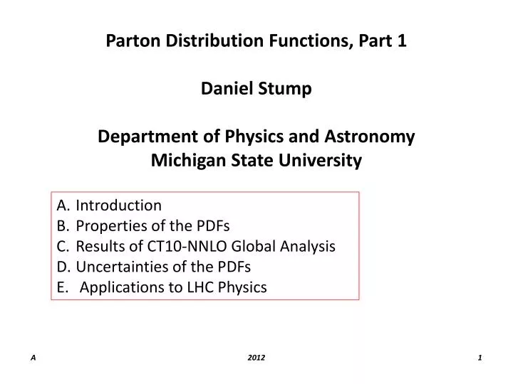
Parton Distribution Functions, Part 1 Daniel Stump Department of Physics and Astronomy Michigan State University. Introduction Properties of the PDFs Results of CT10-NNLO Global Analysis Uncertainties of the PDFs Applications to LHC Physics. Introduction.

E N D
Parton Distribution Functions, Part 1 Daniel Stump Department of Physics and Astronomy Michigan State University Introduction Properties of the PDFs Results of CT10-NNLO Global Analysis Uncertainties of the PDFs Applications to LHC Physics 2012
Introduction A. Introduction. QCD and High-Energy Physics QCD is an elegant theory of the strong interactions – the gauge theory of color transformations. It has a simple Lagrangian (sums over flavor and color are implied) Parameters: g; m1, m2, m3, …, m6 2012
Introduction However, the calculation of experimental observables is quite difficult, for 2 reasons: (i) there are divergent renormalizations; the theory requires • regularization • perturbation theory • a singular limit • L (GeV) • or, a 0 (fm) • or, n 4 (ii) quark confinement; the asymptotic states are color singlets, whereas the fundamental fields are color triplets. 2012
Introduction • Nevertheless, certain cross sections can be calculated reliably --- • --- inclusive processes with large momentum transfer (i.e., short-distance interactions) • The reasons that QCD can provide accurate predictions for short-distance interactions are • asymptotic freedom • as(Q2) ~ const./ln(Q2/L2) as Q2 • the factorization theorem • dshadron~ PDFs C • where C is calculable in perturbation theory. • The PDFs provide a connection between quarks and gluons (the partons) and the nucleon (a bound state). 2012
Introduction Global Analysis of QCD and Parton Distribution Functions dshadron~ PDFs C (sum over flavors implied) The symbol ~ means “asymptotically equal as Q ”; the error is O(m2/Q2) where Q is an appropriate (high) momentum scale. The C’s are calculable in perturbation theory. The PDFs are not calculable today, given our lack of understanding of the nonperturbative aspect of QCD (binding and confinement). But we can determine the PDFs from Global Analysis, with some accuracy. 2012
next … 2012
Properties of the PDFs B. Properties of the PDFs -- Definitions First, what are the Parton Distribution Functions? (PDFs) The PDFs are a set of 11 functions, fi (x,Q2) where longitudinal momentum fraction momentum scale parton index f0 = g(x,Q2) the gluon PDF f1 = u(x,Q2) the up-quark PDF f-1 = u(x,Q2) the up-antiquark PDF f2 = d and f-2 = d f3 = s and f-3 = s etc. - - Exercise: What about the top quark? - 2012
Properties of the PDFs Second, what is the meaning of a PDF? We tend to think and speak in terms of “Proton Structure” u(x,Q2) dx = the mean number of up quarks with longitudinal momentum fraction from x to x + dx, appropriate to a scattering experiment with momentum transfer Q. u(x,Q2) = the up-quark density in momentum fraction This heuristic interpretation makes sense from the LO parton model. More precisely, taking account of QCD interactions, dsproton = PDFs C . 2012
Properties of the PDFs fi(x,Q2) = the density of parton type i w.r.t. longitudinal momentum fraction x Momentum Sum Rule longitudinal momentum fraction, carried by parton type i Flavor Number Sum Rules valence up quark integral, valence down quark integral, valence strange quark integral 2012
Properties of the PDFs Example. DIS of electrons by protons; e.g., HERA experiments in lowest order of QCD (summed over flavors!) 2012
Properties of the PDFs But QCD radiative corrections must be included to get a sufficiently accurate prediction. The NLO approximation will involve these interactions … From these perturbative calculations, we determine the coefficient functions Ci(NLO), and hence write Approximations available today: LO, NLO, NNLO 2012
Properties of the PDFs Correlator function The Factorization Theorem For short-distance interactions, and thePDFsareuniversal! We can write a formal, field-theoretic expression, although we can’t evaluate it because we don’t know the bound state |p>. 2012
Properties of the PDFs Exercise. Suppose the parton densities for the proton are known, (A) In terms of the fi(x,Q2), write the 11 parton densities for the neutron, say, gi(x,Q2). (B) In terms of the fi(x,Q2), write the 11 parton densities for the deuteron, say, hi(x,Q2). 2012
next … 2012
Q2 evolution Q2 evolution B. Properties of the PDFs – Q2 evolution Evolution in Q The PDFs are a set of 11 functions, fi(x,Q2)where longitudinal momentum fraction momentum scale fi(x,Q2) = the density of partons of type i, carrying a fraction x of the longitudinal momentum of a proton, when resolved at a momentum scale Q. • The DGLAP Evolution Equations • We know how the fivary with Q. • That follows from the renormalization group. • It’s calculable in perturbation theory . 2012
Q2 evolution Q2 evolution The DGLAP Evolution Equations V.N. Gribov and L.N. Lipatov, Sov J Nucl Phys 15, 438 (1972); G. Altarelli and G. Parisi, Nucl Phys B126, 298 (1977); Yu.L. Dokshitzer, Sov Phys JETP 46, 641 (1977). Solve the 11 coupled equations numerically. For example, you could download the program HOPPET. G. P. Salam and J. Rojo, A Higher Order Perturbative Parton Evolution Toolkit; download from http://projects.hepforge.org/hoppet … a library of programs written in Fortran 90. 2012
Q2 evolution 2012
Q2 evolution Q2 evolution Some informative results obtained using HOPPET Starting from a set of “benchmark input PDFs”, let’s use HOPPET to calculate the evolved PDFs at selected values of Q. For the input (not realistic but used here to study the evolution qualitatively): Output tables 2012
Q2 evolution Q2 evolution The Running Coupling of QCD aS(Q2) 2012
Q2 evolution Q2 evolution The QCD Running Coupling Constant For Global Analysis, we need an accurate aS(Q2). (approx. : NF = 5 massless) 2012
Q2 evolution Q2 evolution The QCD Running Coupling Constant • Evolution of aS as a function of Q, using • the 1-loop beta function (red) • the 2-loop beta function (green) • the 3-loop beta function (blue) For Global Analysis, we need an accurate aS(Q2). aS(MZ) = 0.11840.0007 S. Bethke, G. Dissertori and G.P. Salam; Particle Data Group 2012 2012
Q2 evolution Q2 evolution The QCD Running Coupling Constant How large are the 2-loop and 3-loop corrections for aS(Q2)? 2012
Q2 evolution Q2 evolution • Comments on aS(Q2) • An important improvement is to include the quark masses. • The central fit has aS(MZ) = 0.118.(Bethke) • CTEQ also provides alternative PDFs with a range of value of aS(MZ); these are called theaS-series. • Another approach is to use the Global Analysis to “determine” the value of aS(MZ). • Asymptotic freedom 2012
Q2 evolution Q2 evolution How does the u-quark PDF evolve in Q? Examples from HOPPET U-quark PDF evolution : Black : Q = Q0 = 1.414 GeV Blue : Q = 3.16 GeV (1-loop, 2-loop, 3-loop) Red : Q = 100.0 GeV (1-loop, 2-loop, 3-loop) 2012
Q2 evolution Q2 evolution How does the gluon PDF evolve in Q? Examples from HOPPET Gluon PDF evolution : Black : Q = Q0 = 1.414 GeV Blue : Q = 3.16 GeV (1-loop, 2-loop, 3-loop) Red : Q = 100.0 GeV (1-loop, 2-loop, 3-loop) 2012
Q2 evolution Q2 evolution DGLAP evolution of PDFs • The “structure of the proton” depends on the resolving power of the scattering process. As Q increases … • PDFs decrease at large x • PDFs increase at small x • as we resolve the gluon radiation and quark pair production. • The momentum sum rule and the flavor sum rules hold for all Q. • These graphs show the DGLAP evolution for LO, NLO, NNLO Global Analysis. 2012
Q2 evolution Q2 evolution How large are the NLO and NNLO corrections? … a good exercise using HOPPET 2012
Q2 evolution Q2 evolution next … 2012
CT10-NNLO PDFs Structure of the Proton CTEQ Parton Distribution Functions CTEQ6.6 P. M. Nadolsky, H.-L. Lai, Q.-H. Cao, J. Huston, J. Pumplin, D. Stump, W.-K. Tung, C.-P. Yuan, Implications of CTEQ global analysis for collider observables, Phys.Rev.D78:013004 (2008) ; arXiv:0802.0007 [hep-ph] CT10 Hung-Liang Lai, Marco Guzzi, Joey Huston, Zhao Li, Pavel M. Nadolsky, Jon Pumplin, C.-P. Yuan, New parton distributions for collider physics, Phys.Rev.D82:074024 (2010) ; arXiv:1007.2241 [hep-ph] CT10-NNLO (2012) The results shown below are for CT10-NNLO. 2012
CT10-NNLO PDFs Structure of the Proton The U Quark (Q2 = 10 GeV2; Q = 3.16 GeV) Red: u(x,Q2) Dashed Red: ū(x,Q2) Gray: uvalence(x,Q2) This log-log plot shows … … for x ≳ 0.1 the valence structure dominates … for x ≲ 0.01 ū approaches u 2012
CT10-NNLO PDFs Structure of the Proton The U Quark (Q2 = 10 GeV2; Q = 3.16 GeV) Red: x u(x,Q2) Dashed Red: x ū(x,Q2) Gray: x uvalence(x,Q2) This linear plot shows the momentum fraction for Q = 3.16 GeV (= area under the curve) integral ≈ 0.32, 0.05, 0.27 2012
CT10-NNLO PDFs Structure of the Proton The U Quark (Q2 = 10 GeV2; Q = 3.16 GeV) Red: uvalence(x,Q2) This linear plot demonstrates the flavor sum rule: integral = 2 2012
CT10-NNLO PDFs Structure of the Proton The D Quark (Q2 = 10 GeV2; Q = 3.16 GeV) Blue: d(x,Q2) Dashed Blue: đ(x,Q2) Gray: dvalence(x,Q2) This log-log plot shows … … for x ≳ 0.1 the valence structure dominates … for x ≲ 0.01 đ approaches d 2012
CT10-NNLO PDFs Structure of the Proton The D Quark (Q2 = 10 GeV2; Q = 3.16 GeV) Blue: d(x,Q2) Dashed Blue: đ(x,Q2) Gray: dvalence(x,Q2) This linear plot shows the momentum fraction for Q = 3.16 GeV (= area under the curve) integral ≈ 0.15, 0.06, 0.10 2012
CT10-NNLO PDFs Structure of the Proton The D Quark (Q2 = 10 GeV2; Q = 3.16 GeV) dvalence = d – đ (x,Q2) This linear plot demonstrates the flavor sum rule: integral = 1 2012
CT10-NNLO PDFs Structure of the Proton The D and U Quarks (Q2 = 10 GeV2; Q = 3.16 GeV) Blue: d(x,Q2) Dashed Blue: đ(x,Q2) Gray: dvalence(x,Q2) Red: u(x,Q2) Dashed Red: ū(x,Q2) Gray: uvalence(x,Q2) This linear plot compares U and D -- quarks and antiquarks; naively, d = 0.5 u, but it’s not that simple. 2012
CT10-NNLO PDFs Structure of the Proton The D and U Quarks (Q2 = 10 GeV2; Q = 3.16 GeV) d(x,Q2) / u(x,Q2) v x d(x,Q2) / u(x,Q2) is interesting. Exercise: What scattering processes could provide information on this ratio? 2012
CT10-NNLO PDFs Structure of the Proton Gluons (Q2 = 10 GeV2; Q = 3.16 GeV) black : g(x,Q2) red : u(x,Q2) The gluon dominates at small x. The valence quarks dominate at large x. 2012
CT10-NNLO PDFs Structure of the Proton Gluons (Q2 = 10 GeV2; Q = 3.16 GeV) black : g(x,Q2) red : u(x,Q2) blue: d(x,Q2) The gluon dominates at small x. The valence quarks dominate at large x. 2012
CT10-NNLO PDFs Structure of the Proton Sea Quarks and Gluons (Q2 = 10 GeV2; Q = 3.16 GeV) sea(x,Q2) and g(x,Q2) vs x black: g(x,Q2) brown: sea(x,Q2) sea = 2 (db + ub + sb) 2012
CT10-NNLO PDFs Structure of the Proton (Q2 = 10 GeV2; Q = 3.16 GeV) Ratios : (db, ub, sb)/g Exercises: (1) Identify db, ub, sb. (2) Why are they all equal at small x? 2012
CT10-NNLO PDFs Structure of the Proton (Q2 = 10 GeV2; Q = 3.16 GeV) All in One Plot u_valence d valence sea * 0.05 gluon * 0.05 Sea = 2 (db + ub + sb) u_valence = u – ub ; u = u_valence + u_sea ub = u_sea 2012
CT10-NNLO PDFs Structure of the Proton … as a function of Q All in One Plot u_valence d valence sea * 0.05 gluon * 0.05 Sea = 2 (db + ub + sb) u_valence = u – ub ; u = u_valence + u_sea ub = u_sea 2012
CT10-NNLO PDFs Exercise: (A) Use the Durham Parton Distribution Generator (online PDF calculator) to reproduce these graphs. (B) Show the Q2 evolution. 2012
next … 2012