Download
1 / 30
300 likes | 480 Views
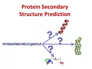
A simple and fast secondary structure prediction method with hidden neural networks. Authors: Kuang Lin, Victor A. Simossis, Willam R. Taylor and Jaap Heringa Presented by: Rashmi Singh Sowmya Tirukkovaluru. Motivation. We introduce a secondary structure prediction method

E N D
Asimple and fast secondary structure prediction method with hidden neural networks Authors: Kuang Lin, Victor A. Simossis, Willam R. Taylor and Jaap Heringa Presented by: Rashmi Singh Sowmya Tirukkovaluru
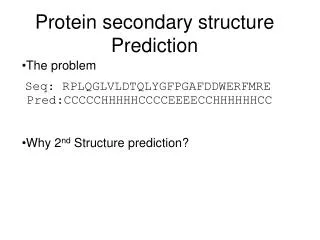
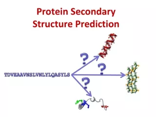
Motivation • We introduce a secondary structure prediction method • called YASPIN. • YASPIN uses a single neural network for predicting the • secondary structure elements in a 7-state local structure • scheme (Hb, H, He, C, Eb, E and Ee) . • Optimizes the output using a hidden Markov model. • Results • YASPIN was compared with the current secondary • structure prediction methods, such as PHDpsi, PROFsec, • JNET, SSPro2, and PSIPRED. • YASPIN shows the highest accuracy in terms of Q3 and • SOV scores for strand prediction.
HISTORY • Qian and Sejnowski (1988) introduced one of the earliest • artificial neural network based methods which use • single sequence as input. • From the 1990’s upto the present time, secondary • structure prediction accuracy has improved to over 70% • by using the evolutionary information found in MSA. • MSA unlike single sequence input, offers a much improved • means to recognise positional physiochemical features • such as hydrophobicity patterns. • However, the improvement in the secondary structure • prediction accuracy by using MSA’s is also directly • connected to database size and search accuracy.
PSI-BLAST • The top-performing methods till date, PHD, PHDpsi, • PROFSec, SSPro2, JNET, PSIPRED use various types • of neural networks for prediction and employ the • database-searching tool PSI-BLAST with same search • parameters • In YASPIN, all sequences were sequentially used as • queries in PSI-BLAST search . • PSI-BLAST is a position specific Iterative BLAST • technique and generates a profile of homologues • sequences in the form of position specific scoring • matrices (PSSM). • All involved secondary structure prediction methods were • tested on the same PSI-BLAST results to make the • comparison as unbiased as possible
YASPIN • Uses a single Neural Network in contrast with many other • NN-based methods which use feed forward-multilayer • perceptron networks, which are trained using back • propagation algorithm • Back-propagation algorithm • 1) Feed forward from Input to output. • 2) Calculate and back-propagate the error (the difference • between the network output and the target output). • 3) Adjust weights in steepest descent direction along the • error surfaceto decrease the error. • w (t+1)= w (t) - r [∂E/∂w] + μ * Δw(t-1) • where r is a positive constant called learning rate, • and μ is the momentum term.
YASPIN • The problem with using single NN method is that its • predictions results are broken secondary structure elements, • even elements of one residue. • This is not desirable as most observed secondary structures • are composed of more than three residues . • In YASPIN, we overcome this problem by using Hidden • Markov model to filter the predicted secondary structure • elements from the NN. • Finally, prediction results are converted into 3-state • secondary structure predictions • (H-Helix, E-Strand, and ‘-’ Other).
Algorithm • YASPINuses a single feed forward perceptron network • with one hidden layer. • YASPIN NN uses the softmax transition function with a • window of 15 residues. Input function: Ak = ∑j Wj xj . soft max activation function: X1 Activation function W1 x2 W2 ∑jWjxj g o Output Wn Input function xn Input links where k’ is the kth ouput unit
Algorithm • For each residue in the window, 20 units are used for • scores in the PSSM( In PSSM ,each column is a vector of • 20 specifying the frequencies of 20 amino acids appearing • in that column of MSA) and 1 unit to mark where the • window spans the terminals of protein chains. • The input layer has 21*15 = 315 units. • Hidden layer has 15 units. • Output layer has 7 units corresponding to seven • local structure states: helix beginning (Hb), Helix (H), • Helix ending (He), Strand beginning (Eb), Strand (E), • Strand ending (Ee) ,coil (C) .
State Diagram • The 7-state output of the NN is passed through a HMM . • It uses viterbi algorithm to optimally segment the • 7-state predictions
Test and training datasets • YASPIN was trained and tested using the SCOP1.65 • (structural classification of proteins) database. • PDB25 was constructed in which the maximal pairwise identity • was limited to 25% making it a non-redundant set. • All transmembrane entries (they do not have structural • information) were removed from the PDB25 resulting in a set of • 4256 proteins with known structures. • The test and training sets were built using the PDB25 set • grouped together by ASTRAL(it.
PDB 25 test set • TEST SET: The test set was extracted before training by • random selection by complete PDB25 at a ratio of about • 1:8. • The 535 sequences selected for the test set were • at most 25% identical to the training set due to the nature • of PDB25 dataset. • Were not part of the same superfamily as any of the • remaining 3721 sequences of the training set.
EVA5 sequence set • EVA5 is the independent ‘common_set 5’ dataset from • EVA consisting of 217 sequences. • To make a more accurate comparison between all methods • including YASPIN, we further benchmarked all methods on • EVA5. • The final YASPIN training set set contained 3553 sequences • with known structures, after removing all sequences found in • the EVA5 sequenceset.
NN Training • On-line back-propagation algorithm and 6-fold cross- • validation is used to train YASPIN Neural Network. • In a single iteration, each of the 6 subsets was used • for testing and the remaining 5 are used for training • NN. • At the end of each iteration, the average prediction • error of the networks over all the six test subsets was • recorded. • The training was stopped when the average • prediction error started increasing. • A momentum term of 0.5 and a learning rate of • 0.0001 was used.
HMM Training • The Secondary structure states used to train the HMM • are obtained using DSSP. • The DSSP 8-state secondary structure • representation(H,G,E,B,I,S,T,-) was grouped according • to the 3 state scheme • (H and G) as Helix(H) • (E and B) as Strand(E) and • others as Coil(C). • These 3 state definitions were then converted into 7 • state local structure scheme.
Reliability scores • YASPIN provides four different position-specific prediction confidence • scores which are generated based on the NN-predicted probabilities • of each residue being in one of the 7 states . • The first 3 scores are secondary structure specific scores, • representing Helix,Strand and Coil prediction confidence and are • generated as a sum of probabilities of each respective secondary • structure type.They are normalized to 9. • The fourth score is the position-specific prediction confidence number • ,which represents the score of the state the viterbi algorithm has • chosen in its optimal segmentation path.
Prediction Accuracy Scores • Q3: Qi = (number of residues correctly predicted in state i / • number of residues observed in state I) * 100 SOV: Segment Overlap quantity measure for a single conformational state SOV(i) = 1 MINOV(S1;S2) + DELTA(S1;S2) • ------ SUM ---------------------------------------------- * LEN(S1) • N(i) MAXOV(S1;S2) • S(i) • MCC:
Testing with PDB25 test set • The 535 sequences of PDB25 test set were used to compare YASPIN to current top performing methods. • 409 sequences were found to be common to all methods • This comparison was relatively unfair for YASPIN since many of these state of the art methods have used sequences from this test set for their training . • YASPIN is the best in strand prediction and also out performs most methods in Helix prediction,except SSPro2 and PSIPRED which are clearly superior to YASPIN.
The average Q3 and SOV scores for the predictions of 409 PDB25 Common sequences from the testing set
Testing with EVA5 test set • EVA 5 sequences were removed from the YASPIN training set and • also from other methods. • From the 217 sequences in the EVA 5 test set, 188 were found to be • common for all methods. • The Q3 prediction accuracy results for separate SSEs showed that • PSIPRED and SSOPro2 were best in the prediction of helix, while • YASPIN was better than all remaining methods • In addition, YASPIN was better at strand prediction.
The average Q3 and SOV scores for the prediction of 188 Common sequences from the EVA 5 set
Calculating prediction errors • Prediction errors for helix and strand are classified into 4 types: • Wrong Prediction (w) • Over Prediction (o) • Under-prediction (u) • Length-errors (l)
Different error types and MCCs for YASPIN • Investigation of errors made by all methods on EVA 5 test set showed • that • All methods are missing out strand segments at the same rate • (EU) • 2) PSIPRED and SSPro2 more frequently over-predict, while rest • under-predict, helix segments (Ho/Hu) • 3) YASPIN mistakes helics for strand (HW), over-elongating strand • segments (Elo) and keeping helices too short (Hlu) • MCCs showed that YASPIN and PROFsec are equivalent in prediction • quality, which suggests that the prediction error types made by each • method are not accurately reflected in Q3 and SOV scores
Investigation of types of errors • All the methods are more or less missing out strand segments at the • same rate –EU • PSIPRED and SSPro2 more frequently over-predict while others under- • predict helix segment – Ho/Hu • YASPIN prediction mistakes helices for strand – HW, over-elongated • strand segments – Elo, and keep helices too short - Hlu
The extent of errors made by each method on independent EVA5 common data set H/EW :wrong prediction H/EO: overprediction H/EU:underprediction H/Elo: length overprediction H/Elu: length underprediction
YASPIN position specific reliability measures • The reliability scoring scheme applied in YASPIN correlated well with • the Q3. • The relationship between the assigned reliability scores and their • corresponding average prediction accuracy (Q3) was almost linear. • This means the YASPIN confidence scoring scheme accurately • describes the reliability of each prediction. • In approx. 48% of the predicted residues, showing confidence value • of 5 or greater, 90% were accurately predicted.
Q3 and the percentage of residues against cumulative Reliability index from the YASPIN method Reliability (greater or equal to value shown)
DISCUSSION • The difference YASPIN and other classical NN-based programs is the • HNN model • In YASPIN, the NN and HMM components of the HNN model were • trained separately while in other approaches they were trained in • combination. • In YASPIN, the initial predictions are 7- state predictions of protein local • structures, instead of commonly used 3 states. • The importance is that the termini of SSEs, esp., Helices, have • statistically significant different composition from other parts of • the protein sequence. • Hence, the network used in the YASPIN is trained to capture these • differences and provide additional information by producing these • 7-state predictions
DISCUSSION • The problem with our model is that the strands predicted by YASPIN • must be of at least 3 residues but according to DSSP definition, • β bridges can have only one residue. • To overcome this problem, two different Markov Models were • designed, each having fewer states of strand structures than those • currently used (Eb, E and Ee), but there is a decrease in the • prediction accuracy • This suggests that the sequence signal of the strand termini are • important for the prediction.