Download
1 / 31
310 likes | 1.41k Views
CHAPTER 4 Species Diversity. Tables, Figures, and Equations. From: McCune, B. & J. B. Grace. 2002. Analysis of Ecological Communities . MjM Software Design, Gleneden Beach, Oregon http://www.pcord.com. Alpha diversity : diversity in individual sample units

E N D
CHAPTER 4 Species Diversity Tables, Figures, and Equations From: McCune, B. & J. B. Grace. 2002. Analysis of Ecological Communities.MjM Software Design, Gleneden Beach, Oregon http://www.pcord.com
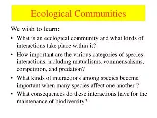
Alpha diversity: diversity in individual sample units • Beta diversity: amount of compositional variation in a sample (a collection of sample units) • Gamma diversity: overall diversity in a collection of sample units, often "landscape-level" diversity
Proportionate diversity measures For an observed abundance xi, (numbers, biomass, cover, etc.) of species i in a sample unit, let pi = proportion of individuals belonging to species i: • a = constant that can be assigned and alters the property of the measure • S = number of species • Da = diversity measure based on the constant a. The units are "effective number of species" Can think of a as the weight given to dominance of a species.
Figure 4.1. Influence of equitability on Hill's (1973a) generalized diversity index. Diversity is shown as a function of the parameter a for two cases: a sample unit with strong inequitability in abundance and a sample unit with perfect equitability in abundance (all species present have equal abundance; see Table 4.1).
D0 = species richness When a = 0, Da is simply species richness.
D2 and Simpson's index Simpson’s (1949) original index (1/D2) is a measure of dominance rather than diversity The complement of Simpson's index of dominance is and is a measure of diversity. It is the likelihood that two randomly chosen individuals will be different species.
D1 and Shannon-Wiener index If a = 1 then D1 is a nonsense equation because the exponent is 1/0. But if we use limits to define D1 as a approaches 1 then
The logarithmic form of D1 is the Shannon-Wiener index (H’), which measures the “information content” of a sample unit: The units for D1 are "number of species of equal abundance“ The units for H' are the log of the number of species of equal abundance.
Box 4.1. How is information related to uncertainty? For plot 1 For plot 2
Table 4.2. Some measures of beta diversity. See Wilson and Mohler (1983) and Wilson and Shmida (1984) for other published methods. “DCA” is detrended correspondence analysis. A direct gradient refers to sample units taken along an explicitly measured environmental or temporal gradient. Indirect gradients are gradients in species composition along presumed environmental gradients
Figure 4.2. Example of rate of change, R, measured as proportional dissimilarity in species composition at different sampling positions along an environmental gradient. Peaks represent relatively abrupt change in species composition. This data set is a series of vegetation plots over a low mountain range. In more homogeneous vegetation, the curve and peaks would be lower.
The amount of change, b, is the integral of the rate of change: where a and b refer to the ends of an ecological gradient x.
Figure 4.3. Hypothetical decline in similarity in species composition as a function of separation of sample units along an environmental gradient, measured in half changes. Sample units one half change apart have a similarity of 50%.
Wilson and Mohler (1983) introduced "gleasons" as a unit of species change. This measures the steepness of species response curves. It is the sum of the slopes of individual species at each point along the gradient. where Y is the abundance of species i at position x along the gradient. This can be integrated into an estimate of beta diversity along a whole gradient with where PS(a,b) is the percentage similarity of sample units a and b and IA is the expected similarity of replicate samples (the similarity intercept on Fig. 4.3).
Minchin measured beta diversity using the mean range of the species’ physiological response function: where ri is the range of species i along the gradient, L is the length of the gradient, and r and L are measured in the same units.
Oksanen and Tonteri (1995) proposed the following measure of total gradient length: where A is the absolute compositional turnover (rate of change) of the community between points a and b on gradient x.
This semi-log plot is the basis for Whittaker's (1960) method of calculating the number of half changes along the gradient segment from a to b, HC(a,b): • where • PS(a,b) is the percentage similarity of sample units a and b • IA is the expected similarity of replicate samples (the y intercept on the figure just described).
Beta turnover measures the amount of change as the "number of communities." where g = the number of species gained, l = the number of species lost = the average species richness in the sample units:
The simplest descriptor of beta diversity and one that can be applied to any community sample, is where is the landscape-level diversity and is the average diversity in a sample unit. Whittaker (1972) stated that a generally appropriate measure of this is where w is the beta diversity, Sc is the number of species in the composite sample (the number of species in the whole data set), and S is the average species richness in the sample units.
As a rule of thumb: • w < 1 is low • 1 < w< 5 is medium • w > 5 is high
Half changes corresponding to the average dissimilarity among sample units: This can be rewritten as Figure 4.4. Conversion of average dissimilarity, measured with a proportion coefficient, to beta diversity measured in half changes (D).
First-order jackknife estimator (Heltshe & Forrester 1983, Palmer 1990) • where • S = the observed number of species, • r1 = the number of species occurring in only one sample unit, and • n = the number of sample units.
The second-order jackknife estimator (Burnham & Overton 1979; Palmer 1991) is: where r2 = the number of species occurring in exactly two sample units.
Evenness An easy-to-use measure (Pielou 1966, 1969) is "Pielou's J" • where • H' is the Shannon-Wiener diversity measure • S is the average species richness. • If there is perfect equitability then log(S) = H' and J = 1.
Hayek and Buzas (1997) partitioned H' into richness and evenness components based on the equation • where • E = eH'/S • e is the base of the natural logarithms.
Figure 4.5. Species-area curve (heavy line) used to assess sample adequacy, based on repeated subsampling of a fixed sample (in this case containing 92 sample units and 122 species). Dotted lines represent 1 standard deviation. The distance curve (light line) describes the average Sørensen distance between the subsamples and the whole sample, as a function of subsample size.
Species – Area equations • Arrhenius (1921): • where • S is the number of species, • A is the area of the sample, and • c and b are fitted coefficients. • In log form:
Table 4.3. Species diversity of epiphytic macrolichens in the southeastern United States. Alpha, beta, and gamma diversity are defined in the text (table from McCune et al. 1997).