Download

1 / 57
590 likes | 623 Views
The Maximum Network Flow Problem. Network Flow. Instance: A Network is a directed graph G Edges represent pipes that carry flow Each edge <u,v> has a maximum capacity c <u,v> A source node s in which flow arrives A sink node t out which flow leaves. Goal: Max Flow. The Problem.

E N D
Network Flow • Instance: • A Network is a directed graph G • Edges represent pipes that carry flow • Each edge <u,v> has a maximum capacity c<u,v> • A source node sin which flow arrives • A sink node t out which flow leaves Goal: Max Flow COSC 3101B, PROF. J. ELDER
The Problem • Use a graph to model material that flows through conduits. • Each edge represents one conduit, and has a capacity, which is an upper bound on the flow rate = units/time. • Can think of edges as pipes of different sizes. • Want to compute max rate that we can ship material from a designated source to a designated sink. COSC 3101B, PROF. J. ELDER
What is a Flow Network? • Each edge (u,v) has a nonnegative capacity c(u,v). • If (u,v) is not in E, assume c(u,v)=0. • We have a source s, and a sink t. • Assume that every vertex v in V is on some path from s to t. • c(s,v1)=16; c(v1,s)=0; c(v2,v3)=0 COSC 3101B, PROF. J. ELDER
What is a Flow in a Network? • For each edge (u,v), the flow f(u,v) is a real-valued function that must satisfy 3 conditions: • Note that skew symmetry condition implies that f(u,u)=0. COSC 3101B, PROF. J. ELDER
capacity flow capacity Example of a Flow: • f(v2, v1) = 1, c(v2, v1) = 4. • f(v1, v2) = -1, c(v1, v2) = 10. • f(v3, s) + f(v3, v1) + f(v3, v2) + f(v3, v4) + f(v3, t) = 0 + (-12) + 4 + (-7) + 15 = 0 COSC 3101B, PROF. J. ELDER
The Value of a flow • The value of a flow is given by • This is the total flow leaving s = the total flow arriving in t. COSC 3101B, PROF. J. ELDER
Example: |f| = f(s, v1) + f(s, v2) + f(s, v3) + f(s, v4) + f(s, t) = 11 + 8 + 0 + 0 + 0 = 19 |f|= f(s, t) + f(v1, t) + f(v2, t) + f(v3, t) + f(v4, t) = 0 + 0 + 0 + 15 + 4 = 19 COSC 3101B, PROF. J. ELDER
A flow in a network • We assume that there is only flow in one direction at a time. • Sending 7 trucks from Edmonton to Calgary and 3 trucks from Calgary to Edmonton has the same net effect as sending 4 trucks from Edmonton to Calgary. COSC 3101B, PROF. J. ELDER
Multiple Sources Network • We have several sources and several targets. • Want to maximize the total flow from all sources to all targets. • Reduce to max-flow by creating a supersource and a supersink: COSC 3101B, PROF. J. ELDER
Residual Networks • The residual capacity of a network with a flow f is given by: • The residual network of a graph G induced by a flow f is the graph including only the edges with positive residual capacity, i.e., COSC 3101B, PROF. J. ELDER
Network: Residual Network: Example of Residual Network COSC 3101B, PROF. J. ELDER
Augmenting Paths • An augmenting pathp is a simple path from s to t on the residual network. • We can put more flow from s to t through p. • We call the maximum capacity by which we can increase the flow on p the residual capacity of p. COSC 3101B, PROF. J. ELDER
Network: Residual Network: Augmenting path Augmenting Paths The residual capacity of this augmenting path is 4. COSC 3101B, PROF. J. ELDER
Ford-Fulkerson Method COSC 3101B, PROF. J. ELDER
End of Lecture 18 November 7, 2006
Flow(1) Residual(1) No more augmenting paths max flow attained. Flow(2) Residual(2) Example COSC 3101B, PROF. J. ELDER
Cuts of Flow Networks COSC 3101B, PROF. J. ELDER
The Net Flow through a Cut (S,T) • f(S,T) = 12 – 4 + 11 = 19 COSC 3101B, PROF. J. ELDER
The Capacity of a Cut (S,T) • c(S,T)= 12+ 0 + 14 = 26 COSC 3101B, PROF. J. ELDER
Augmenting Paths – example • The maximum possible flow through the cut = 12 + 7 + 4 = 23 Flow(2) cut The network has a capacity of at most 23. This is called a minimum cut. COSC 3101B, PROF. J. ELDER
Net Flow of a Network • The net flow across any cut is the same and equal to the flow of the network |f|. COSC 3101B, PROF. J. ELDER
Bounding the Network Flow • The value of any flow f in a flow network G is bounded from above by the capacity of any cut of G. COSC 3101B, PROF. J. ELDER
Max-Flow Min-Cut Theorem • If f is a flow in a flow network G=(V,E), with source s and sink t, then the following conditions are equivalent: • f is a maximum flow in G. • The residual network Gf contains no augmented paths. • |f| = c(S,T) for some cut (S,T) (a min-cut). COSC 3101B, PROF. J. ELDER
The Basic Ford-Fulkerson Algorithm COSC 3101B, PROF. J. ELDER
augmenting path Original Network Resulting Flow = Example 4 COSC 3101B, PROF. J. ELDER
4 augmenting path Residual Network Resulting Flow = Example COSC 3101B, PROF. J. ELDER
Example Residual Network Resulting Flow = 11 COSC 3101B, PROF. J. ELDER
Resulting Flow = 11 augmenting path Residual Network Example COSC 3101B, PROF. J. ELDER
Residual Network Resulting Flow = Example 19 COSC 3101B, PROF. J. ELDER
Resulting Flow = 19 augmenting path Residual Network Example COSC 3101B, PROF. J. ELDER
Residual Network Resulting Flow = Example 23 COSC 3101B, PROF. J. ELDER
Resulting Flow = 23 No augmenting path: Maxflow=23 Residual Network Example COSC 3101B, PROF. J. ELDER
O(E) O(E) Analysis COSC 3101B, PROF. J. ELDER
Analysis • If capacities are all integer, then each augmenting path raises |f| by ≥ 1. • If max flow is f*, then need ≤ |f*| iterations time is O(E|f*|). • Note that this running time is not polynomial in input size. It depends on |f*|, which is not a function of |V| or |E|. • If capacities are rational, can scale them to integers. • If irrational, FORD-FULKERSON might never terminate! COSC 3101B, PROF. J. ELDER
The Basic Ford-Fulkerson Algorithm • With time O ( E |f*|), the algorithm is not polynomial. • This problem is real: Ford-Fulkerson may perform very badly if we are unlucky: |f*|=2,000,000 COSC 3101B, PROF. J. ELDER
Run Ford-Fulkerson on this example Augmenting Path Residual Network COSC 3101B, PROF. J. ELDER
Run Ford-Fulkerson on this example Augmenting Path Residual Network COSC 3101B, PROF. J. ELDER
Run Ford-Fulkerson on this example • Repeat 999,999 more times… COSC 3101B, PROF. J. ELDER
The Edmonds-Karp Algorithm • A small fix to the Ford-Fulkerson algorithm makes it work in polynomial time. • Specify how to compute the path in line 4. COSC 3101B, PROF. J. ELDER
The Edmonds-Karp Algorithm • Compute the path in line 4 using breadth-first search on residual network. • The augmenting path p is the shortest path from s to t in the residual network (treating all edge weights as 1). • Runs in time O(V E2). COSC 3101B, PROF. J. ELDER
The Edmonds-Karp Algorithm - example • Edmonds-Karp’s algorithm halts in only 2 iterations on this graph. COSC 3101B, PROF. J. ELDER
Further Improvements • Push-relabel algorithm ([CLRS, 26.4]) – O(V2 E). • The relabel-to-front algorithm ([CLRS, 26.5) – O(V3). • (We will not cover these) COSC 3101B, PROF. J. ELDER
Maximum Bipartite Matching • A bipartite graph is a graph G=(V,E) in which V can be divided into two parts L and R such that every edge in E is between a vertex in L and a vertex in R. • e.g. vertices in L represent skilled workers and vertices in R represent jobs. An edge connects workers to jobs they can perform. COSC 3101B, PROF. J. ELDER
A matching in a graph is a subset M of E, such that for all vertices v in V, at most one edge of M is incident on v. COSC 3101B, PROF. J. ELDER
A maximummatching is a matching of maximum cardinality. maximum not maximum COSC 3101B, PROF. J. ELDER
A Maximum Matching • No matching of cardinality 4, because only one of v and u can be matched. • In the workers-jobs example a max-matching provides work for as many people as possible. v u COSC 3101B, PROF. J. ELDER
Solving the Maximum Bipartite Matching Problem • Reduce an instance of the maximum bipartite matching problem on graph G to an instance of the max-flow problem on a corresponding flow network G’. • Solve using Ford-Fulkerson method. COSC 3101B, PROF. J. ELDER
Corresponding Flow Network • To form the corresponding flow network G' of the bipartite graph G: • Add a source vertex s and edges from s to L. • Direct the edges in E from L to R. • Add a target vertex t and edges from R to t. • Assign a capacity of 1 to all edges. • Claim: max-flow in G’ corresponds to a max-bipartite-matching on G. COSC 3101B, PROF. J. ELDER
min cut Example |M| = 3 max flow = 3 COSC 3101B, PROF. J. ELDER