Download
1 / 13
130 likes | 134 Views
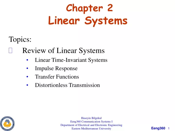
Chapter 2 Linear Systems. Topics: Review of Linear Systems Linear Time-Invariant Systems Impulse Response Transfer Functions Distortionless Transmission. Huseyin Bilgekul Eeng360 Communication Systems I Department of Electrical and Electronic Engineering

E N D
Chapter 2 Linear Systems Topics: • Review of Linear Systems • Linear Time-Invariant Systems • Impulse Response • Transfer Functions • Distortionless Transmission Huseyin Bilgekul Eeng360 Communication Systems I Department of Electrical and Electronic Engineering Eastern Mediterranean University
Linear Time-Invariant Systems • An electronic filter or system is Linearwhen Superpositionholds, that is when, • Where y(t) is the output and x(t) = a1x1(t)+a2x2(t) is the input. • l[.] denotes the linear (differential equation) system operator acting on [.]. • If the system is time invariant for any delayed input x(t – t0), the output is delayed by just the same amount y(t – t0). • That is, the shape of the response is the same no matter when the input is applied to the system.
Impulse Response x(t)
Transfer Function • The output waveform for a time-invariant network can be obtained by convolving the input waveform with the impulse response of the system. • The impulse response can be used to characterize the response of the system in the time domain. • The spectrum of the output signal is obtained by taking the Fourier transform of both sides. Using the convolution theorem, • Where H(f) = ℑ[h(t)] is transfer function orfrequency responseof the network. • The impulse response and frequency response are a Fourier transform pair: • Generally, transfer function H(f)is a complex quantity and can be written in polar form.
The |H(f)|is the Amplitude (or magnitude) Response. • The Phase Response of the network is Transfer Function • Since h(t)is a real function of time (for real networks), it follows • |H(f)|is an even function of frequency and • θ(f)is an odd function of frequency.
Power Transfer Function • It is possible to derive the relationship between the power spectral density (PSD) at the input, Px(f), and that at the output, Py(f) , of a linear time-invariant network. Using the definition of PSD PSD of the output is Using transfer function in a formal sense, we obtain Thus, the power transfer function of the network is
Example 2.14 RC Low Pass Filter 3dB Point
Distortionless Transmission No Distortion if y(t)=Ax(t-Td) Y(f)=AX(f)e-j2fTd • Distortionless channel implies that channel output is proportional to delayed version of input • For no distortion at the output of an LTI system, two requirements must be satisfied: • The amplitude response is flat. • |H(f)| = Constant = A( No Amplitude Distortion) • The phase response is a linear function of frequency. • θ(f) = <H(f) = -2πfTd(No Phase Distortion) Second requirement is often specified equivalently by using the time delay. We define the time delayof the system as: • If Td(f) is not constant, there is phase distortion, Because the phase response θ(f), is not a linear function of frequency.
Example 2.15 Distortion Caused By an RC filter • For f <0.5f0, the filter will provide almost distortionless transmission. The error in the magnitude response is less than 0.5 dB. The error in the phase is less than 2.18 (8%). • For f <f0, The error in the magnitude response is less than 3 dB. The error in the phase is less than 12.38 (27%). • In engineering practice, this type of error is often considered to be tolerable.
Example 2.15 Distortion Caused By a filter • The magnitude response of the RC filter is not constant. • Distortion is introduced to the frequencies in the pass band below frequency fo.
Example 2.15 Distortion Caused By a filter • The phase response of the RC filter is not a linear function of frequency. • Distortion is introduced to the frequencies in the pass band below frequency fo. • The time delay across the RC filter is not constant for all frequencies. • Distortion is introduced to the frequencies in the pass band below frequency fo.