Download
1 / 31
310 likes | 439 Views
Experts Learning and The Minimax Theorem for Zero-Sum Games. December 8th 2011. Maria Florina Balcan. Motivation. Many situations involve repeated decision making. Deciding how to invest your money (buy or sell stocks). What route to drive to work each day.

E N D
Experts Learning and The Minimax Theorem for Zero-Sum Games December 8th 2011 Maria Florina Balcan
Motivation Many situations involve repeated decision making • Deciding how to invest your money (buy or sell stocks) • What route to drive to work each day • Playing repeatedly a game against an opponent with unknown strategy This course: Learning algos for such settings with connections to game theoretic notions of equilibria
Roadmap Last lecture: Online learning; combining expert advice; the Weighted Majority Algorithm. This lecture: Online learning, game theory, minimax optimality.
Recap: Online learning, minimizing regret, and combining expert advice. • “The weighted majority algorithm” N. Littlestone & M. Warmuth • “Online Algorithms in Machine Learning” (survey) A. Blum • Algorithmic Game Theory, Nisan, Roughgarden, Tardos, Vazirani (eds) [Chapters 4]
Online learning, minimizing regret, and combining expert advice. Expert 3 Expert 2 Expert 1
Using “expert” advice Assume we want to predict the stock market. • Will the market go up or down? • We solicit n “experts” for their advice. • We then want to use their advice somehow to make our prediction. E.g., Can we do nearly as well as best in hindsight? Note: “expert” ´ someone with an opinion. [Not necessairly someone who knows anything.]
Formal model • For each round t=1,2, …, T • There are n experts. • Each expert makes a prediction in {0,1} • The learner (using experts’ predictions) makes a prediction in {0,1} • The learner observes the actual outcome. There is a mistake if the predicted outcome is different form the actual outcome. Can we do nearly as well as best in hindsight?
Weighted Majority Algorithm Key Point: A mistake doesn't completely disqualify an expert. Instead of crossing off, just lower its weight. Weighted Majority Algorithm • Start with all experts having weight 1. • Predict based on weighted majority vote. • If • then predict 1 • else predict 0
Weighted Majority Algorithm Key Point: A mistake doesn't completely disqualify an expert. Instead of crossing off, just lower its weight. Weighted Majority Algorithm • Start with all experts having weight 1. • Predict based on weighted majority vote. • Penalize mistakes by cutting weight in half.
Analysis: do nearly as well as best expert in hindsight Theorem: If M = # mistakes we've made so far and OPT = # mistakes best expert has made so far, then:
Randomized Weighted Majority 2.4(OPT + lg n)not so good if the best expert makes a mistake 20% of the time. Can we do better? • Yes.Instead of taking majority vote, use weights as probabilities. (e.g., if 70% on up, 30% on down, then pick 70:30) Key Point: smooth out the worst case. • Also, generalize ½ to 1- e. Equivalent to select an expert with probability proportional with its weight.
Formal Guarantee for Randomized Weighted Majority Theorem: If M = expected # mistakes we've made so far and OPT = # mistakes best expert has made so far, then: • M ·(1+e)OPT + (1/e) log(n)
Randomized Weighted Majority Solves to:
Summarizing • E[# mistakes] ·(1+e)OPT + e-1log(n). • If set =(log(n)/OPT)1/2 to balance the two terms out (or use guess-and-double), get bound of • E[mistakes]·OPT+2(OPT¢log n)1/2 Note: Of course we might not know OPT, so if running T time steps, since OPT · T, set ² to get additive loss (2T log n)1/2 regret • E[mistakes]·OPT+2(T¢log n)1/2 • So, regret/T ! 0. [no regret algorithm]
What if have n options, not n predictors? • We’re not combining n experts, we’re choosing one. • Can we still do it? • Nice feature of RWM: can be applied when experts are n different options • E.g., n different ways to drive to work each day, n different ways to invest our money. • We did not see the predictions in order to select an expert (only needed to see their losses to update our weights)
Decision Theoretic Version; Formal model • For each round t=1,2, …, T • There are n experts. • No predictions. The learner produces a prob distr. on experts based on their past performance pt. • The learner is given a loss vector lt and incurs expected loss lt¢ pt. • The learner updates the weights. The guarantee also applies to this model!!! [Interesting for connections between GT and Learning.]
Can generalize to losses in [0,1] • If expert i has loss li, do: wià wi(1-li). [before if an expert had a loss of 1, we multiplied by (1-epsilon), if it had loss of 0 we left it alone, now we do linearly in between] • Same analysis as before.
This lecture: Online Learning, Game Theory, and Minimax Optimality “Game Theory, On-line Prediction, and Boosting”, Freund & Schapire, GEB
Zero Sum Games Game defined by a matrix M. Assume wlog entries are in [0,1]. Scissors Rock Paper 1/2 1 0 Rock Paper 0 1/2 1 Row player (Mindy) chooses row i. Scissors 1 0 1/2 Column player (Max) chooses column j (simultaneously). Mindy’s goal: minimize her loss M(i,j). Max’s goal: maximize this loss (zero sum).
Randomized Play Mindy chooses a distribution P over rows. Max chooses a distribution Q over columns [simultaneously] Mindy’s expected loss: If i,j = pure strategies, and P,Q = mixed strategies M(P,j) - Mindy’s expected loss when she plays P and Max plays j M(i,Q) - Mindy’s expected loss when she plays i and Max plays Q
Sequential Play Say Mindy plays before Max. If Mindy chooses P, then Max will pick Q to maximize M(P,Q), so the loss will be So, Mindy should pick P to minimize L(P). Loss will be: Similarly, if Max plays first, loss will be:
Minimax Theorem Playing second cannot be worse than playing first Mindy plays first Mindy plays second Von Neumann’s minimax theorem: No advantage to playing second! Regardless of who goes first the outcome is always the same!
Optimal Play Von Neumann’s minimax theorem: Value of the game Optimal strategies: Min-max strategy Max-min strategy 1. Even if Max knows Mindy’s strategy, Max cannot get better outcome than v. v is the best possible value. 9 min-max strategy P*s.t. for any Q, M(P*,Q) · v. 2. No matter what strategy Mindy uses, the outcome is at worst v. 9 max-min strategy Q*s.t. for any P, M(P, Q*) ¸ v.
Optimal Play Von Neumann’s minimax theorem: Value of the game Optimal strategies: Min-max strategy Max-min strategy P*and Q*optimal strategies if the opponent is also optimal! For a two person zero-sum game against a good opponent, your best bet is to find your min-max optimal strategy and always play it.
Optimal Play Von Neumann’s minimax theorem: Value of the game Optimal strategies: Min-max strategy Max-min strategy Note: (P*, Q*) is a Nash equilibrium. P*is a best response to Q*; Q*is a best response to P* All the NE have the same value in zero-sum games. Not true in general, very specific to zero-sum games!!!
Optimal Play Von Neumann’s minimax theorem: Value of the game Optimal strategies: Min-max strategy Max-min strategy P*and Q*optimal strategies if the opponent is also optimal! For a two person zero-sum game against a good opponent, your best bet is to find your min-max optimal strategy and always play it.
Beyond the Classic Theory Often limited info about the game or the opponent • M maybe unknown or very large. • Opponent may not be fully adversarial. Bart Simpson always plays Rock instead of choosing the uniform distribution. You can play Paper and always beat Bart. As game is played over and over, opportunity to learn the game and/or the opponent’s strategy.
Repeated Play • For each round t=1,2, …, T Exactly fits DT experts model! • M unknown. • Mindy chooses Pt • Max chooses Qt (possibly based on Pt) • Mindy’s loss is M(Pt, Qt) = Pt ¢ (MQt) • Mindy observes loss M(i, Qt) for each pure strategy i. lt= MQt Mindy can run RWM to ensure: minPM(P,(Q1+…+QT)/T) · v where
Prove minimax theorem as corollary Need to prove: [¸ part is trivial ] Imaging game is played repeatedly. In each round t Mindy plays using RWM Max chooses best response Define:
One slide proof of minimax theorem is a strategy that you can use if you have to go first.