Download
1 / 55
550 likes | 642 Views
Lecture 8 The Principle of Maximum Likelihood. Syllabus.

E N D
Syllabus Lecture 01 Describing Inverse ProblemsLecture 02 Probability and Measurement Error, Part 1Lecture 03 Probability and Measurement Error, Part 2 Lecture 04 The L2 Norm and Simple Least SquaresLecture 05 A Priori Information and Weighted Least SquaredLecture 06 Resolution and Generalized Inverses Lecture 07 Backus-Gilbert Inverse and the Trade Off of Resolution and VarianceLecture 08 The Principle of Maximum LikelihoodLecture 09 Inexact TheoriesLecture 10 Nonuniqueness and Localized AveragesLecture 11 Vector Spaces and Singular Value Decomposition Lecture 12 Equality and Inequality ConstraintsLecture 13 L1 , L∞ Norm Problems and Linear ProgrammingLecture 14 Nonlinear Problems: Grid and Monte Carlo Searches Lecture 15 Nonlinear Problems: Newton’s Method Lecture 16 Nonlinear Problems: Simulated Annealing and Bootstrap Confidence Intervals Lecture 17 Factor AnalysisLecture 18 Varimax Factors, Empircal Orthogonal FunctionsLecture 19 Backus-Gilbert Theory for Continuous Problems; Radon’s ProblemLecture 20 Linear Operators and Their AdjointsLecture 21 Fréchet DerivativesLecture 22 Exemplary Inverse Problems, incl. Filter DesignLecture 23 Exemplary Inverse Problems, incl. Earthquake LocationLecture 24 Exemplary Inverse Problems, incl. Vibrational Problems
Purpose of the Lecture • Introduce the spaces of all possible data, • all possible models and the idea of likelihood Use maximization of likelihood as a guiding principle for solving inverse problems
Part 1The spaces of all possible data,all possible models and the idea of likelihood
viewpoint the observed data is one point in the space of all possible observations or dobs is a point in S(d)
plot of dobs d3 d2 d1 O
plot of dobs d3 d2 dobs d1 O
now suppose … the data are independent each is drawn from a Gaussian distribution with the same mean m1 and variance σ2 (but m1 and σ unknown)
plot of p(d) d3 d2 d1 O
plot of p(d) d3 cloud centered on d1=d2=d3 with radius proportional to σ d2 d1 O
now interpret … p(dobs) as the probability that the observed data was in fact observed L = log p(dobs) called the likelihood
find parameters in the distribution maximize p(dobs) with respect to m1 and σ maximize the probability that the observed data were in fact observed the Principle of Maximum Likelihood
solving the two equations usual formula for the sample mean almost the usual formula for the sample standard deviation
these two estimates linked to the assumption of the data being Gaussian-distributed might get a different formula for a different p.d.f.
example of a likelihood surface L(m1, σ) maximum likelihood point σ m1
likelihood maximization process will fail if p.d.f. has no well-defined peak (A) (B) p(d1, ,d1 ) p(d1, ,d1 ) d2 d2 d1 d1
Part 2Using the maximization of likelihood as a guiding principle for solving inverse problems
linear inverse problem for with Gaussian-distibuted datawith known covariance [covd]assumeGm=dgives the mean d T
principle of maximum likelihoodmaximize L = log p(dobs)minimize T with respect to m
principle of maximum likelihoodmaximize L = log p(dobs)minimize T E = This is just weighted least squares
principle of maximum likelihoodwhen data Gaussian-distributedsolve Gm=d with weighted least squareswith weighting of
special case of uncorrelated dataeach datum with a different variance[covd]ii = σdi2minimize
special case of uncorrelated dataeach datum with a different variance[covd]ii = σdi2minimize errors weighted by their certainty
probabilistic representation of a priori information probability that the model parameters are near m given by p.d.f. pA(m)
probabilistic representation of a priori information probability that the model parameters are near m given by p.d.f. pA(m) centered at a priori value <m>
probabilistic representation of a priori information probability that the model parameters are near m given by p.d.f. pA(m) variance reflects uncertainty in a priori information
uncertain certain <m2> <m2> m2 m2 <m1> <m1> m1 m1
<m2> m2 <m1> m1
linear relationship approximation with Gaussian <m2> m2 m2 <m1> m1 m1
m2 p=constant m1 p=0
assessing the information contentin pA(m) Do we know a little about m or a lot about m ?
Information Gain, S • -S called Relative Entropy,
Relative Entropy, Salso called Information Gain null p.d.f. state of no knowledge
Relative Entropy, Salso called Information Gain uniform p.d.f. might work for this
probabilistic representation of data probability that the data are near d given by p.d.f. pA(d)
probabilistic representation of data probability that the data are near d given by p.d.f. p(d) centered at observed data dobs
probabilistic representation of data probability that the data are near d given by p.d.f. p(d) variance reflects uncertainty in measurements
probabilistic representation of both prior information and observed data assume observations and a priori information are uncorrelated
Example of map model,m dobs datum,d
the theoryd = g(m)is a surface in the combined space of data and model parameterson which the estimated model parameters and predicted data must lie
the theoryd = g(m)is a surface in the combined space of data and model parameterson which the estimated model parameters and predicted data must liefor a linear theorythe surface is planar
the principle of maximum likelihood says maximize on the surface d=g(m)
(A) model,m dobs dpre d=g(m) datum,d map mest (B) p(s) smax position along curve,s
model,m dobs dpre d=g(m) datum,d mest≈map p(s) smax position along curve,s
(A) model,m dpre≈dobs d=g(m) datum,d map mest (B) p(s) position along curve,s smax
minimize principle of maximum likelihoodwithGaussian-distributed dataGaussian-distributed a priori information
this is just weighted least squareswith so we already know the solution