Download
1 / 22
250 likes | 864 Views
Chapter 6: Bounded Aquifers. Stephanie Fulton January 24, 2014. What is a bounded aquifer?. Either confined or unconfined Bounded on one or more sides by either a Recharging boundary (e.g., river or canal) Barrier boundary (e.g., impermeable valley wall)

E N D
Chapter 6: Bounded Aquifers Stephanie Fulton January 24, 2014
What is a bounded aquifer? • Either confined or unconfined • Bounded on one or more sides by either a • Recharging boundary (e.g., river or canal) • Barrier boundary (e.g., impermeable valley wall) • Aquifer pump tests must sometimes be conducted near one or more types of boundaries • Invalidates the assumption that the aquifer is of “infinite areal extent” • The use of image wells and the “principle of superposition” are applied to transform an aquifer of finite areal extent into one of seemingly infinite extent which allows the use of methods from previous chapters
Types of Bounded Aquifers Barrier Boundary Recharging Boundary
Steady State Flow: Dietz’s Method • One or more recharge boundaries (Fig. 6.2) • Uses several different Green’s functions to describe the influence of the boundaries • Solution describes the impulse response of an ODE with specified initial conditions or boundary conditions (Wikipedia: http://en.wikipedia.org/wiki/Green's_function) • Assumptions • Same as for confined aquifer EXCEPT: • Aquifer can be either confined OR unconfined • Within the pumping influence zone, aquifer is crossed by one or more straight, fully penetrating recharge boundaries with a constant water level • The hydraulic contact between the recharge boundaries and the aquifer is as permeable as the aquifer • Flow to the well is in steady state
Image Wells • Positioned such that that pumping well and image well form mirror images of one another: • Located on the opposite side of boundary from the pumping well • At the exact distance away from boundary as the pumping well • Recharge boundary: image well is a recharge well • Barrier boundary: image well is a discharge well • Flow rate is always constant, and is equal to the rate of the real pumping well • By using the law of superposition (i.e., the drawdown from two or more wells can be added to find the resulting overall drawdown) the drawdown from the real well and the image well will give you the actual drawdown • More than one boundary? More than one image well will be needed
Steady State: Dietz’s Method • Uses Green’s functions to describe the influence of the boundaries • Depending on what kind of boundaries are present determines which G(x,y) to use:
Dietz’s Method: Green functions • One straight recharge boundary (Figure 6.2A):
Dietz’s Method: Green Functions (cont.) • Two straight recharge boundaries at right angles to each other (Fig. 6.2B):
Dietz’s Method: Green Functions (cont.) • Two straight parallel recharge boundaries (Fig. 6.2C):
Dietz’s Method: Green Functions (cont.) • U-shaped recharge boundary (Fig. 6.2D):
Unsteady State: Stallman’s Method • One or more straight recharge or barrier boundaries • The distance between the real well and a piezometer is r; the distance between an image well and the piezometer is ri and their ratio is ri/r = rr • The number of terms between the brackets (Eq. 6.8) depends on how many image wells there are: • If there is only one image well, there are two terms between the brackets • W(u) describes the influence of the real well, and the others (i.e., W(rr2u)) represent the image wells • Values of W(rr2u) provided in Annex 6.1 • A discharge well (real or image) gives terms with a positive sign • A recharge well gives terms with a negative sign
Unsteady State Flow: Stallman’s Method (cont.) • Assumptions are the same as for Dietz’s method EXCEPT flow to the well is in unsteady state • Equation 6.8 is based Theis’ well function for confined aquifers but is applicable to unconfined aquifers as long as Assumption 7 (Ch. 3) is not violated (e.g., no apparent delay in water table response) • Method:
Unsteady State: Hantush’s Method • One recharge boundary • Useful when the effective line of recharge does not correspond with the bank or the streamline of the river or canal • Can be compensated for by making the distance between the pumped well and the hydraulic boundary in the equivalent system greater than the distance between the pumped well and actual boundary
Unsteady State: Hantush’s Method (cont.) • Assumptions • Same as for Stalling method EXCEPT: • Within the pumping influence zone, aquifer is crossed by a straight recharge boundary with a constant water level • The resistance between the recharge boundary and the aquifer should be small, but not negligible • It should be possible to extrapolate steady-state drawdown for each piezometer • It is not necessary to know the following beforehand: • z(distance between pumping well and recharge boundary) • location of the image well, nor the distance ridependent on it • ri/r = rr
Unsteady State: Hantush’s Method (cont.) • Much like Stallman’s method, drawdown in an aquifer bounded on one side by a recharge boundary is: • Where: • The relation equation between rr, x, r, and z is given by: 4z2– 4xz – r2(rr2 – 1) = 0 (6.20)
Unsteady State: Hantush’s Method (cont.) • If the drawdown is plotted on semi-log paper versus t (with t on the log scale), there is an inflection point P on the curve. At this point, the value of u is given as: (6.21)
Unsteady State: Hantush’s Method (cont.) • The slope of the curve is: (6.22) • And drawdown is: (6.23) • For values of t > 4tp , the drawdown (s) approaches the maximum drawdown: (6.24) • The ratio of sm (Equation 6.24) and Δsp(Eq. 6.22), depends solely on the value of rr. So (6.25)
Unsteady State: Vandenberg’s Method • Leaky aquifers bounded laterally by two parallel barrier boundaries form an ‘infinite strip aquifer’ • You have to consider not only the boundary effects, but also the leakage effects
Unsteady State: Vandenberg’s Method (cont.) • For x > w (i.e., x/w > 1): • Where
Unsteady State: Vandenberg’s Method (cont.) • Values of the function F(u,x/L) for different values of u and x/L can be plotted as a family of type curves (see Annex 6.5) • With values found from matching the data curve with the type curves, you can use Eq. 6.26 to find T. Then you can use Eq. 6.28 to find S. By knowing x/L and x, you can calculate L. Then from Eq. 6.29 you can find c.
Important Notes: Vandenberg’s Method • When x/L=0 (i.e., when L is ∞) the drawdown function (Eq. 6.26) becomes the same as that for parallel flow in a confined channel aquifer: • If x/w < 1, Eq. 6.26 is not accurate, and the following equation can be used instead: • Type curves can be constructed from this equation, but for each particular configuration of pumped well and piezometer, a different set of curves is required.