Download
1 / 54
550 likes | 673 Views
Graphs and Networks with Bioconductor. Wolfgang Huber EMBL/EBI Bressanone 2005 Based on chapters from "Bioinformatics and Computational Biology Solutions using R and Bioconductor", Gentleman, Carey, Huber, Irizarry, Dudoit, Springer Verlag, to appear Aug 2005. Graphs.

E N D
Graphs and Networks with Bioconductor Wolfgang Huber EMBL/EBI Bressanone 2005 Based on chapters from "Bioinformatics and Computational Biology Solutions using R and Bioconductor", Gentleman, Carey, Huber, Irizarry, Dudoit, Springer Verlag, to appear Aug 2005.
Graphs Set of nodes and set of edges. Nodes: objects of interest Edges: relationships between them A useful abstraction to talk about relationships and interactions (think of integer numbers, apples and fingers) Edges may have weights, directions, types
Practicalities As always, need to distinguish between the true, underlying property of nature that you want to measure, and the actual result of a measurement (experiment) 1. False positive edges 2. False negative edges (were tested, were not found, but are there in nature) 3. Untested edges (were not tested, are not in your data, but are there in nature) Uncertainty is not usually considered in mainstream graph theory, but cannot be ignored in functional genomics. Nice application of these concepts to protein interactions: Gentleman and Scholtens, SAGMB 2004
Representation Node-edge lists Adjacency matrix (straightforward) Adjacency matrix (sparse) From-To matrix They are equivalent, but may be hugely different in performance and convenience for different applications. Can coerce between the representations
Algorithms Bioconductor project emphasizes re-use and interfacing to existing, well-tested software implementations rather than reimplementing everything from scratch ourselves. RBGL package: interface to Boost Graph Library; started by V. Carey, R. Gentleman, now driven by Li Long.
Elementary computations on IMCA pathway > library("graph") > data("integrinMediatedCellAdhesion") > class(IMCAGraph) > s = acc(IMCAGraph, "SOS") Ha-Ras Raf MEK 1 2 3 ERK MYLK MYO 4 5 6 F-actin cell proliferation 7 5
Machine-readable pathway databases KEGG reactome BioCarta (biocarta.com) National Cancer Institute cMAP
Gene Ontology (GO) A structed vocabulary to describe molecular function of gene products, biological processes, and cellular components. Plus A set of "is a", "is part of" relationships between these terms Directed acyclic graph
GO graphs >tfG=GOGraph("GO:0003700", GOMFPARENTS)
Literature graphs DKC1
Graphs: vocabulary Directed, undirected graphs Adjacent nodes Accessible nodes Self-loop Multi-edge Node degree Walk: alternating sequence of nodes and incident edges Closed walk Distance between nodes, shortest walk Trail: walk with no repeated edges Path: trail with no repeated nodes (except possibly first/last) Cycle Connected graph Weakly connected directed graph (see next page)
Graphs: vocabulary Cut: remove edges to disconnect a graph Cut-set: remove nodes - " - Connectivity of a graph Cliques
Bipartite graphs AG adjacency matrix (n x m) of a bipartite graph G with node sets U, V One mode graphs AU = AGt AG AV = AGAGt 0•1=0+0=0•0=0, 0+1=1+1=1•1=1
Multigraphs Can have different types of edges
Hypergraphs := set of Nodes + set of hyperedges A hyperedge is a set of nodes (can be more than 2) A directed hyperedge: pair (tail and head) of sets of nodes
Directed acyclic graphs Useful for representing hierarchies, partial orderings (e.g. in time, from general to special, from cause to effect) Many applications: GO MeSH Graphical models
Random Edge Graphs n nodes, m edges p(i,j) = 1/m with high probability: m < n/2: many disconnected components m > n/2: one giant connected component: size ~ n. (next biggest: size ~ log(n)). degrees of separation: log(n). Erdös and Rényi 1960
Random graphs Random edge graph: randomEGraph(V, p, edges) V: nodes either p: probability per edge or edges: number of edges Random graph with latent factor: randomGraph(V, M, p, weights=TRUE) V: nodes M: latent factor p: probability For each node, generate a logical vector of length length(M), with P(TRUE)=p. Edges are between nodes that share >= 1 elements. Weights can be generated according to number of shared elements. Random graph with predefined degree distribution: randomNodeGraph(nodeDegree) nodeDegree: named integer vector sum of all node degrees must be even
Random edge graph 100 nodes 50 edges degree distribution
Random graphs versus permutation graphs For statistical inference, one can consider null hypotheses based on aforementioned random graph models; and ones based on node permutation of data graphs. The second is often more appropriate.
Cohesive subgroups For data graphs, the concept of clique is usually too restrictive (false negative or untested edges) n-clique: distance between all members is <=n. (Clique: n=1) k-plex: maximal subgraph G in which each member is neighbour of at least |G|-k others. (Clique: k=1) k-core: maximal subgraph G in which each member is neighbour of at least k others. (Clique: k=|G|-1) After: Social Network Analysis, Wasserman and Faust (1994)
graph, RBGL, Rgraphviz graph basic class definitions and functionality RBGL interface to graph algorithms Rgraphviz rendering functionality Different layout algorithms. Node plotting, line type, color etc. can be controlled by the user.
Creating our first graph > library("graph"); library(Rgraphviz) > myNodes = c("s", "p", "q", "r") > myEdges = list( s = list(edges = c("p", "q")), p = list(edges = c("p", "q")), q = list(edges = c("p", "r")), r = list(edges = c("s"))) > g = new("graphNEL", nodes = myNodes, edgeL = myEdges, edgemode = "directed") > plot(g)
Querying nodes, edges, degree > nodes(g) [1] "s" "p" "q" "r" > edges(g) $s [1] "p" "q" $p [1] "p" "q" $q [1] "p" "r" $r [1] "s" > degree(g) $inDegree s p q r 1 3 2 1 $outDegree s p q r 2 2 2 1
adjacent and accessible nodes > adj(g, c("b", "c")) $b [1] "b" "c" $c [1] "b" "d" > acc(g, c("b", "c")) $b a c d 3 1 2 $c a b d 2 1 1
Graph manipulation > g1 <- addNode("e", g) > g2 <- removeNode("d", g) > ## addEdge(from, to, graph, weights) > g3 <- addEdge("e", "a", g1, pi/2) > ## removeEdge(from, to, graph) > g4 <- removeEdge("e", "a", g3) > identical(g4, g1) [1] TRUE
Graph representations: from-to-matrix > ft [,1] [,2] [1,] 1 2 [2,] 2 3 [3,] 3 1 [4,] 4 4 > ftM2adjM(ft) 1 2 3 4 1 0 1 0 0 2 0 0 1 0 3 1 0 0 0 4 0 0 0 1
GXL: graph exchange language <gxl> <graph edgemode="directed" id="G"> <node id="A"/> <node id="B"/> <node id="C"/> … <edge id="e1" from="A" to="C"> <attr name="weights"> <int>1</int> </attr> </edge> <edge id="e2" from="B" to="D"> <attr name="weights"> <int>1</int> </attr> </edge> … </graph> </gxl> GXL (www.gupro.de/GXL) is "an XML sublanguage designed to be a standard exchange format for graphs". The graph package provides tools for im- and exporting graphs as GXL from graph/GXL/kmstEx.gxl
RBGL: interface to the Boost Graph Library Connected components cc = connComp(rg) table(listLen(cc)) 1 2 3 4 15 18 36 7 3 2 1 1 Choose the largest component wh = which.max(listLen(cc)) sg = subGraph(cc[[wh]], rg) Depth first search dfsres = dfs(sg, node = "N14") nodes(sg)[dfsres$discovered] [1] "N14" "N94" "N40" "N69" "N02" "N67" "N45" "N53" [9] "N28" "N46" "N51" "N64" "N07" "N19" "N37" "N35" [17] "N48" "N09" rg
bfs(sg, "N14") depth / breadth first search dfs(sg, "N14")
wc = connComp(g2) connected components sc = strongComp(g2) nattrs = makeNodeAttrs(g2, fillcolor="") for(i in 1:length(sc)) nattrs$fillcolor[sc[[i]]] = myColors[i] plot(g2, "dot", nodeAttrs=nattrs)
shortest path algorithms Different algorithms for different types of graphs o all edge weights the same o positive edge weights o real numbers …and different settings of the problem o single pair o single source o single destination o all pairs Functions bfs dijkstra.sp sp.between johnson.all.pairs.sp
set.seed(123) rg2 = randomEGraph(nodeNames, edges = 100) fromNode = "N43" toNode = "N81" sp = sp.between(rg2, fromNode, toNode) sp[[1]]$path [1] "N43" "N08" "N88" [4] "N73" "N50" "N89" [7] "N64" "N93" "N32" [10] "N12" "N81" sp[[1]]$length [1] 10 1 shortest path
ap = johnson.all.pairs.sp(rg2) hist(ap) shortest path
gr mst = mstree.kruskal(gr) minimal spanning tree
connectivity Consider graph g with single connected component. Edge connectivity of g: minimum number of edges in g that can be cut to produce a graph with two components. Minimum disconnecting set: the set of edges in this cut. > edgeConnectivity(g) $connectivity [1] 2 $minDisconSet $minDisconSet[[1]] [1] "D" "E" $minDisconSet[[2]] [1] "D" "H"
Rgraphviz: the different layout engines dot: directed graphs. Works best on DAGs and other graphs that can be drawn as hierarchies. neato: undirected graphs using ’spring’ models twopi: radial layout. One node (‘root’) chosen as the center. Remaining nodes on a sequence of concentric circles about the origin, with radial distance proportional to graph distance. Root can be specified or chosen heuristically.
ImageMap lg = agopen(g, …) imageMap(lg, con=file("imca-frame1.html", open="w") tags= list(HREF = href, TITLE = title, TARGET = rep("frame2", length(AgNode(nag)))), imgname=fpng, width=imw, height=imh) Show drosophila interaction network example
Combining R graphics and graphviz: custom node drawing functions
Using GO to interprete gene lists Packages: Gostats, Rgraphviz