Download
1 / 70
700 likes | 889 Views
EE360: Multiuser Wireless Systems and Networks Lecture 2 Outline. Announcements HW 0 due Monday (high-impact papers – you decide) Bandwidth Sharing in Multiuser Channels FD, TD, CD, SD, Hybrid (OFDMA) Overview of Multiuser Channel Capacity Capacity of Broadcast Channels

E N D
EE360: Multiuser Wireless Systems and NetworksLecture 2 Outline • Announcements • HW 0 due Monday (high-impact papers – you decide) • Bandwidth Sharing in Multiuser Channels • FD, TD, CD, SD, Hybrid (OFDMA) • Overview of Multiuser Channel Capacity • Capacity of Broadcast Channels • AWGN, Fading, and ISI • Capacity of MAC Channels • Duality between BC and MAC channels • MIMO Channels
Review of Last Lecture • Overview of multiuser wireless systems and networks • Multiuser systems • Cellular, Ad-Hoc, Cognitive, and Sensor Networks • Random Access Techniques • ALOHA • CSMA-CD • Reservation Protocols • Random access works poorly in heavily loaded systems
Code Space Code Space Code Space Time Time Time Frequency Frequency Frequency Deterministic Bandwidth Sharing • Frequency Division • Time Division • Code Division • Multiuser Detection • Space Division (MIMO) • Hybrid Schemes (OFDMA) What is optimal? Look to Shannon.
OFDMA and SDMA • OFDMA • Combines OFDM and frequency division multiplexing • Different subcarriers assigned to different users • SDMA (space-division multiple access) • Different spatial dimensions assigned to different users • Implemented via multiuser beamforming (e.g. zero-force beamforming) • Benefits from multiuser diversity
Code Division viaMultiple Access SS • Interference between users mitigated by code cross correlation • In downlink, signal and interference have same received power • In uplink, “close” users drown out “far” users (near-far problem) a a
Multiuser Detection • In all CDMA systems and in TD/FD/CD cellular systems, users interfere with each other. • In most of these systems the interference is treated as noise. • Systems become interference-limited • Often uses complex mechanisms to minimize impact of interference (power control, smart antennas, etc.) • Multiuser detection exploits the fact that the structure of the interference is known • Interference can be detected and subtracted out • Better have a darn good estimate of the interference
Ideal Multiuser Detection - Signal 1 = Signal 1 Demod Iterative Multiuser Detection A/D A/D A/D A/D Signal 2 Signal 2 Demod - = Why Not Ubiquitous Today? Power and A/D Precision
Multiuser Shannon CapacityFundamental Limit on Data Rates Capacity: The set of simultaneously achievable rates {R1,…,Rn} with arbitrarily small probability of error • Main drivers of channel capacity • Bandwidth and received SINR • Channel model (fading, ISI) • Channel knowledge and how it is used • Number of antennas at TX and RX • Duality connects capacity regions of uplink and downlink R3 R2 R3 R2 R1 R1
Broadcast Channel Capacity Region in AWGN • Model • One transmitter, two receivers with spectral noise density n1, n2: n1<n2. • Transmitter has average power Pand total bandwidth B. • Single User Capacity: • Maximum achievable rate with asymptotically small Pe • Set of achievable rates includes (C1,0) and (0,C2), obtained by allocating all resources to one user.
Rate Region: Time Division • Time Division (Constant Power) • Fraction of time t allocated to each user is varied • Time Division (Variable Power) • Fraction of time t and power siallocated to each user is varied
Rate Region: Frequency Division • Frequency Division • Bandwidth Biand power Siallocated to each user is varied. Equivalent to TD for Bi=tiB and Pi=tisi.
Superposition Coding Best user decodes fine points Worse user decodes coarse points
Code Division • Superposition Coding • Coding strategy allows better user to cancel out interference from worse user. • DS spread spectrum with spreading gain G and cross correlationr12= r21 =G: • By concavity of the log function, G=1 maximizes the rate region. • DS without interference cancellation
Broadcast: One Transmitter to Many Receivers. Wireless Gateway Multiple Access: Many Transmitters to One Receiver. x x x g1(t) g2(t) g3(t) Broadcast and MAC Fading Channels Wired Network R3 R2 R1 Goal: Maximize the rate region {R1,…,Rn}, subject to some minimum rate constraints, by dynamic allocation of power, rate, and coding/decoding. Assume transmit power constraint and perfect TX and RX CSI
Fading Capacity Definitions • Ergodic (Shannon) capacity: maximum long-term rates averaged over the fading process. • Shannon capacity applied directly to fading channels. • Delay depends on channel variations. • Transmission rate varies with channel quality. • Zero-outage (delay-limited*) capacity: maximum rate that can be maintained in all fading states. • Delay independent of channel variations. • Constant transmission rate – much power needed for deep fading. • Outage capacity: maximum rate that can be maintained in all nonoutage fading states. • Constant transmission rate during nonoutage • Outage avoids power penalty in deep fades *Hanly/Tse, IT, 11/98
+ + + + Two-User Fading Broadcast Channel h1[i] n1[i] Y1[i] x X[i] Y2[i] x n2[i] h2[i] At each time i: n={n1[i],n2[i]} n1[i]=n1[i]/h1[i] Y1[i] X[i] Y2[i] n2[i]=n2[i]/h2[i]
Ergodic Capacity Region* • Capacity region: ,where • The power constraint implies • Superposition coding and successive decoding achieve capacity • Best user in each state decoded last • Power and rate adapted using multiuser water-filling: power allocated based on noise levels and user priorities *Li/Goldsmith, IT, 3/01
Zero-Outage Capacity Region* • The set of rate vectors that can be maintained for all channel states under power constraint P • Capacity region defined implicitly relative to power: • For a given rate vector R and fading state n we find the minimum power Pmin(R,n) that supports R. • RCzero(P) if En[Pmin(R,n)] P *Li and Goldsmith, IT, 3/01
Outage Capacity Region • Two different assumptions about outage: • All users turned off simultaneously (common outage Pr) • Users turned off independently (outage probability vector Pr) • Outage capacity region implicitly defined from the minimum outage probability associated with a given rate • Common outage: given (R,n), use threshold policy • IfPmin(R,n)>s* declare an outage, otherwise assign this power to state n. • Power constraint dictates s* : • Outage probability:
Independent Outage • With independent outage cannot use the threshold approach: • Any subset of users can be active in each fading state. • Power allocation must determine how much power to allocate to each state and which users are on in that state. • Optimal power allocation maximizes the reward for transmitting to a given subset of users for each fading state • Reward based on user priorities and outage probabilities. • An iterative technique is used to maximize this reward. • Solution is a generalized threshold-decision rule.
Broadcast Channels with ISI • ISI introduces memory into the channel • The optimal coding strategy decomposes the channel into parallel broadcast channels • Superposition coding is applied to each subchannel. • Power must be optimized across subchannels and between users in each subchannel.
H1(w) H2(w) Broadcast Channel Model w1k • Both H1 and H2are finite IR filters of length m. • The w1kand w2k are correlated noise samples. • For 1<k<n, we call this channel the n-block discrete Gaussian broadcast channel (n-DGBC). • The channel capacity region is C=(R1,R2). xk w2k
0<k<n Circular Channel Model • Define the zero padded filters as: • The n-Block Circular Gaussian Broadcast Channel (n-CGBC) is defined based on circular convolution: where ((.)) denotes addition modulo n.
0<j<n 0<j<n Equivalent Channel Model • Taking DFTs of both sides yields • Dividing by H and using additional properties of the DFT yields ~ where {V1j} and {V2j} are independent zero-mean Gaussian random variables with
Parallel Channel Model V11 Y11 + X1 Y21 + V21 Ni(f)/Hi(f) V1n f Y1n + Xn Y2n + V2n
Channel Decomposition • The n-CGBC thus decomposes to a set of n parallel discrete memoryless degraded broadcast channels with AWGN. • Can show that as n goes to infinity, the circular and original channel have the same capacity region • The capacity region of parallel degraded broadcast channels was obtained by El-Gamal (1980) • Optimal power allocation obtained by Hughes-Hartogs(’75). • The power constraint on the original channel is converted by Parseval’s theorem to on the equivalent channel.
Capacity Region of Parallel Set • Achievable Rates (no common information) • Capacity Region • For 0<b find {aj}, {Pj} to maximize R1+bR2+lSPj. • Let (R1*,R2*)n,b denote the corresponding rate pair. • Cn={(R1*,R2*)n,b : 0<b }, C=liminfnCn . b R2 R1
Multiple Access Channel • Multiple transmitters • Transmitter i sends signal Xiwith power Pi • Common receiver with AWGN of power N0B • Received signal: X1 X3 X2
MAC Capacity Region • Closed convex hull of all (R1,…,RM) s.t. • For all subsets of users, rate sum equals that of 1 superuser with sum of powers from all users • Power Allocation and Decoding Order • Each user has its own power (no power alloc.) • Decoding order depends on desired rate point
Two-User Region Superposition coding w/ interference canc. Time division C2 SC w/ IC and time sharing or rate splitting Ĉ2 Frequency division SC w/out IC Ĉ1 C1
Fading and ISI • MAC capacity under fading and ISI determined using similar techniques as for the BC • In fading, can define ergodic, outage, and minimum rate capacity similar as in BC case • Ergodic capacity obtained based on AWGN MAC given fixed fading, averaged over fading statistics • Outage can be declared as common, or per user • MAC capacity with ISI obtained by converting to equivalent parallel MAC channels over frequency
Comparison of MAC and BC P • Differences: • Shared vs. individual power constraints • Near-far effect in MAC • Similarities: • Optimal BC “superposition” coding is also optimal for MAC (sum of Gaussian codewords) • Both decoders exploit successive decoding and interference cancellation P1 P2
MAC-BC Capacity Regions • MAC capacity region known for many cases • Convex optimization problem • BC capacity region typically only known for (parallel) degraded channels • Formulas often not convex • Can we find a connection between the BC and MAC capacity regions? Duality
Dual Broadcast and MAC Channels Gaussian BC and MAC with same channel gains and same noise power at each receiver x + x + x x + Multiple-Access Channel (MAC) Broadcast Channel (BC)
P1=0.5, P2=1.5 P1=1.5, P2=0.5 The BC from the MAC P1=1, P2=1 Blue = BC Red = MAC MAC with sum-power constraint
Sum-Power MAC • MAC with sum power constraint • Power pooled between MAC transmitters • No transmitter coordination Same capacity region! BC MAC
BC to MAC: Channel Scaling • Scale channel gain by a, power by 1/a • MAC capacity region unaffected by scaling • Scaled MAC capacity region is a subset of the scaled BC capacity region for any a • MAC region inside scaled BC region for anyscaling MAC + + + BC
The BC from the MAC Blue = Scaled BC Red = MAC
Duality: Constant AWGN Channels • BC in terms of MAC • MAC in terms of BC What is the relationship between the optimal transmission strategies?
Transmission Strategy Transformations • Equate rates, solve for powers • Opposite decoding order • Stronger user (User 1) decoded last in BC • Weaker user (User 2) decoded last in MAC
Duality Applies to DifferentFading Channel Capacities • Ergodic (Shannon) capacity: maximum rate averaged over all fading states. • Zero-outage capacity: maximum rate that can be maintained in all fading states. • Outage capacity: maximum rate that can be maintained in all nonoutage fading states. • Minimum rate capacity: Minimum rate maintained in all states, maximize average rate in excess of minimum Explicit transformations between transmission strategies