Download
1 / 47
490 likes | 741 Views
Chapter 4 Data Preprocessing. To make data more suitable for data mining. To improve the data mining analysis with respect to time, cost and quality. Why Data Preprocessing?. Data in the real world is dirty

E N D
Chapter 4Data Preprocessing To make data more suitable for data mining. To improve the data mining analysis with respect to time, cost and quality.
Why Data Preprocessing? • Data in the real world is dirty • incomplete: missing attribute values, lack of certain attributes of interest, or containing only aggregate data • e.g., occupation=“” • noisy: containing errors or outliers • e.g., Salary=“-10” • inconsistent: containing discrepancies in codes or names • e.g., Age=“42” Birthday=“03/07/1997” • e.g., Was rating “1,2,3”, now rating “A, B, C” • e.g., discrepancy between duplicate records
Why Is Data Preprocessing Important? • No quality data, no quality mining results! • Quality decisions must be based on quality data • e.g., duplicate or missing data may cause incorrect or even misleading statistics. • Data preparation, cleaning, and transformation comprises the majority of the work in a data mining application (90%).
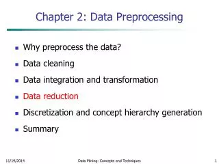
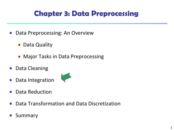
Major Tasks in Data Preprocessing(Fig 3.1) • Data cleaning • Fill in missing values, smooth noisy data, identify or remove outliers and noisy data, and resolve inconsistencies • Data integration • Integration of multiple databases, or files • Data transformation • Normalization and aggregation • Data reduction • Obtains reduced representation in volume but produces the same or similar analytical results • Data discretization (for numerical data)
Data Cleaning • Importance • “Data cleaning is the number one problem in data warehousing” • Data cleaning tasks – this routine attempts to • Fill in missing values • Identify outliers and smooth out noisy data • Correct inconsistent data • Resolve redundancy caused by data integration
Missing Data • Data is not always available • E.g., many tuples have no recorded values for several attributes, such as customer income in sales data • Missing data may be due to • equipment malfunction • inconsistent with other recorded data and thus deleted • data not entered due to misunderstanding • certain data may not be considered important at the time of entry • not register history or changes of the data
How to Handle Missing Data? • Ignore the tuple • Class label is missing (classification) • Not effective method unless several attributes missing values • Fill in missing values manually: tedious (time consuming) + infeasible (large db)? • Fill in it automatically with • a global constant : e.g., “unknown”, a new class?! (misunderstanding)
Cont’d • the attribute mean • Average income of AllElectronics customer $28,000 (use this value to replace) • The attribute mean for all samples belonging to the same class as the given tuple • the most probable value • determined with regression, inference-based such as Bayesian formula, decision tree. (most popular)
Noisy Data • Noise: random error or variance in a measured variable. • Incorrect attribute values may due to • faulty data collection instruments • data entry problems • data transmission problems • etc • Other data problems which requires data cleaning • duplicate records, incomplete data, inconsistent data
How to Handle Noisy Data? • Binning method: • first sort data and partition into (equi-depth) bins • then one can smooth by bin means, smooth by bin median, smooth by bin boundaries, etc. • Clustering • Similar values are organized into groups (clusters). • Values that fall outside of clusters considered outliers. • Combined computer and human inspection • detect suspicious values and check by human (e.g., deal with possible outliers) • Regression • Data can be smoothed by fitting the data to a function such as with regression. (linear regression/multiple linear regression)
Binning Methods for Data Smoothing • Sorted data for price (in dollars): 4, 8, 15, 21, 21, 24, 25, 28, 34 • Partition into (equi-depth) bins: • Bin 1: 4, 8, 15 • Bin 2: 21, 21, 24 • Bin 3: 25, 28, 34 • Smoothing by bin means: • Bin 1: 9, 9, 9 • Bin 2: 22, 22, 22 • Bin 3: 29, 29, 29 • Smoothing by bin boundaries: • Bin 1: 4, 4, 15 • Bin 2: 21, 21, 24 • Bin 3: 25, 25, 34
Outlier Removal • Data points inconsistent with the majority of data • Different outliers • Valid: CEO’s salary, • Noisy: One’s age = 200, widely deviated points • Removal methods • Clustering • Curve-fitting • Hypothesis-testing with a given model
Data Integration • Data integration: • combines data from multiple sources(data cubes, multiple db or flat files) • Issues during data integration • Schema integration • integrate metadata (about the data) from different sources • Entity identification problem: identify real world entities from multiple data sources, e.g., A.cust-id B.cust-#(same entity?) • Detecting and resolving data value conflicts • for the same real world entity, attribute values from different sources are different, e.g., different scales, metric vs. British units • Removing duplicates and redundant data • An attribute can be derived from another table (annual revenue) • Inconsistencies in attribute naming
Correlation analysis • Can detect redundancies
Cont’d • > 0 , A and B positively correlated • values of A increase as values of B increase • The higher the value, the more each attribute implies the other • High value indicate that A (or B) may be removed as a redundancy • = 0, A and B independent (no correlation) • < 0, A and B negatively correlated • Values of one attribute increase as the values of the other attribute decrease (discourages each other)
Data Transformation • Smoothing: remove noise from data (binning, clustering, regression) • Normalization: scaled to fall within a small, specified range such as –1.0 to 1.0 or 0.0 to 1.0 • Attribute/feature construction • New attributes constructed / added from the given ones • Aggregation: summarization or aggregation operations apply to data • Generalization: concept hierarchy climbing • Low level/ primitive/raw data are replace by higher level concepts
Data Transformation: Normalization • Useful for classification algorithms involving • Neural networks • Distance measurements (nearest neighbor) • Backpropagation algorithm (NN) – normalizing help in speed up the learning phase • Distance-based methods – normalization prevent attributes with initially large range (i.e. income) from outweighing attributes with initially smaller ranges (i.e. binary attribute)
Data Transformation: Normalization • min-max normalization • z-score normalization • normalization by decimal scaling Where j is the smallest integer such that Max(| |)<1
Example: • Suppose that the minimum and maximum values for the attribute income are $12,000 and $98,000, respectively. We would like to map income to the range [0.0, 1.0]. • Suppose that the mean and standard deviation of the values for the attribute income are $54,000 and $16,000, respectively. • Suppose that the recorded values of A range from –986 to 917.
Data Reduction Strategies • Data is too big to work with – may takes time, impractical or infeasible analysis • Data reduction techniques • Obtain a reduced representation of the data set that is much smaller in volume but yet produce the same (or almost the same) analytical results • Data reduction strategies • Data cube aggregation – apply aggregation operations (data cube)
Cont’d • Dimensionality reduction—remove unimportant attributes • Data compression – encoding mechanism used to reduce data size • Numerosity reduction – data replaced or estimated by alternative, smaller data representation - parametric model (store model parameter instead of actual data), non-parametric (clustering sampling, histogram) • Discretization and concept hierarchy generation – replaced by ranges or higher conceptual levels
Data Cube Aggregation • Store multidimensional aggregated information • Provide fast access to precomputed, summarized data – benefiting on-line analytical processing and data mining Fig. 3.4 and 3.5
Dimensionality Reduction • Feature selection (i.e., attribute subset selection): • Select a minimum set of attributes (features) that is sufficient for the data mining task. • Best/worst attributes are determined using test of statistical significance – information gain (building decision tree for classification) • Heuristic methods (due to exponential # of choices – 2d): • step-wise forward selection • step-wise backward elimination • combining forward selection and backward elimination • etc
Decision tree induction • Originally for classification • Internal node denotes a test on an attribute • Each branch corresponds to an outcome of the test • Leaf node denotes a class prediction • At each node – algorithm chooses the ‘best attribute to partition the data into individual classes • In attribute subset selection – it is constructed from given data
Data Compression • Compressed representation of the original data • Original data can be reconstructed from compressed data (without loss of info – lossless, approximate - lossy) • Two popular and effective of lossy method: • Wavelet Transforms • Principle Component Analysis (PCA)
Numerosity Reduction • Reduce the data volume by choosing alternative ‘smaller’ forms of data representation • Two type: • Parametric – a model is used to estimate the data, only the data parameters is stored instead of actual data • regression • log-linear model • Nonparametric –storing reduced representation of the data • Histograms • Clustering • Sampling
Regression • Develop a model to predict the salary of college graduates with 10 years working experience • Potential sales of a new product given its price • Regression - used to approximate the given data • The data are modeled as a straight line. • A random variable Y (response variable), can be modeled as a linear function of another random variable, X (predictor variable), with the equation
Cont’d • Y is assumed to be constant • and (regression coefficients) – Y-intercept and the slope line. • Can be solved by the method of least squares. (minimizes the error between actual line separating data and the estimate of the line)
Multiple regression • Extension of linear regression • Involve more than one predictor variable • Response variable Y can be modeled as a linear function of a multidimensional feature vector. • Eg: multiple regression model based on 2 predictor variables X1 and X2
A popular data reduction technique Divide data into buckets and store average (sum) for each bucket Use binning to approximate data distributions Bucket – horizontal axis, height (area) of bucket – the average frequency of the values represented by the bucket Bucket for single attribute-value/frequency pair – singleton buckets Continuous ranges for the given attribute Histograms
Example • A list of prices of commonly sold items (rounded to the nearest dollar) • 1,1,5,5,5,5,5,8,8,10,10,10,10,12, 14,14,14,15,15,15,15,15,15,18,18,18,18,18,18,18,18,18,20,20,20,20,20,20,20,21,21,21,21,25,25,25,25,25,28,28,30,30,30. Refer Fig. 3.9
Cont’d • How are the bucket determined and the attribute values partitioned? (many rules) • Equiwidth, Fig. 3.10 • Equidepth • V-Optimal – most accurate & practical • MaxDiff – most accurate & practical
Clustering • Partition data set into clusters, and one can store cluster representation only • Can be very effective if data is clustered but not if data is “smeared”/ spread • There are many choices of clustering definitions and clustering algorithms. We will discuss them later.
Sampling • Data reduction technique • A large data set to be represented by much smaller random sample or subset. • 4 types • Simple random sampling without replacement (SRSWOR). • Simple random sampling with replacement (SRSWR). • Develop adaptive sampling methods such as cluster sample and stratified sample Refer Fig. 3.13 pg 131
Discretization and Concept Hierarchy • Discretization • reduce the number of values for a given continuous attribute by dividing the range of the attribute into intervals. Interval labels can then be used to replace actual data values • Concept hierarchies • reduce the data by collecting and replacing low level concepts (such as numeric values for the attribute age) by higher level concepts (such as young, middle-aged, or senior)
Discretization • Three types of attributes: • Nominal — values from an unordered set • Ordinal — values from an ordered set • Continuous — real numbers • Discretization: • divide the range of a continuous attribute into intervals because some data mining algorithms only accept categorical attributes. • Some techniques: • Binning methods – equal-width, equal-frequency • Histogram • Entropy-based methods
Binning • Attribute values (for one attribute e.g., age): • 0, 4, 12, 16, 16, 18, 24, 26, 28 • Equi-width binning – for bin width of e.g., 10: • Bin 1: 0, 4 [-,10) bin • Bin 2: 12, 16, 16, 18 [10,20) bin • Bin 3: 24, 26, 28 [20,+) bin • – denote negative infinity, + positive infinity • Equi-frequency binning – for bin density of e.g., 3: • Bin 1: 0, 4, 12 [-, 14) bin • Bin 2: 16, 16, 18 [14, 21) bin • Bin 3: 24, 26, 28 [21,+] bin
Entropy-based discretization • Information-based measure – entropy • Recursively partition the values of a numeric attribute (hierarchical discretization) • Method: Given a set of tuples, S, basic method for entropy-based discretization of A (attribute) is as follows:
Cont’d • Each value of A can be considered a potential interval boundary or threshold T. For example, a value v of A can partition the samples in S into two subsets satisfying the condition A < v and A >= v – binary discretization • Given S, the threshold value selected if the one that maximizes the information gain resulting from subsequent partitioning.
Information gain S1 and S2 – the samples in S satisfying the condition A < T and A >=T
Entropy function • Ent for a given set is calculated based on the class distribution of the samples in the set. Eg, given m classes, the entropy of S1 is Pi– probability of class i in S1, determined by dividing the number of samples of class i in S1 by the total number of samples in S1
Entropy-based (1) • Given attribute-value/class pairs: • (0,P), (4,P), (12,P), (16,N), (16,N), (18,P), (24,N), (26,N), (28,N) • Entropy-based binning via binarization: • Intuitively, find best split so that the bins are as pure as possible • Formally characterized by maximal information gain. • Let S denote the above 9 pairs, p=4/9 be fraction of P pairs, and n=5/9 be fraction of N pairs. • Entropy(S) = - p log p - n log n. • Smaller entropy – set is relatively pure; smallest is 0. • Large entropy – set is mixed. Largest is 1.
Entropy-based (2) • Let v be a possible split. Then S is divided into two sets: • S1: value <= v and S2: value > v • Information of the split: • I(S1,S2) = (|S1|/|S|) Entropy(S1)+ (|S2|/|S|) Entropy(S2) • Goal: split with maximal information gain. • Possible splits: mid points b/w any two consecutive values.
Cont. • For v=14 I(S1,S2) = 0 + 6/9*Entropy(S2) = 6/9 * 0.65 = 0.433 • The best split is found after examining all possible splits. Try for v 16, find I(S1,S2) ? • The process of determining a threshold value is recursively applied until the following stopping criteria • The above example no more splitting because S1&S@ contains purely class, i.e., all P and all N
Summary • Data preparation is a big issue for data mining • Data preparation includes • Data cleaning and data integration • Data reduction and feature selection • Discretization • Many methods have been proposed but still an active area of research