1 / 0

Chapter 5 SUPPLY

Chapter 5 SUPPLY. I. WHAT IS SUPPLY?. The energy crisis of the 1970s encouraged countries to look to nuclear reactors, fueled by

tola
Download Presentation

Chapter 5 SUPPLY

An Image/Link below is provided (as is) to download presentation Download Policy: Content on the Website is provided to you AS IS for your information and personal use and may not be sold / licensed / shared on other websites without getting consent from its author. Content is provided to you AS IS for your information and personal use only. Download presentation by click this link. While downloading, if for some reason you are not able to download a presentation, the publisher may have deleted the file from their server. During download, if you can't get a presentation, the file might be deleted by the publisher.

E N D

Presentation Transcript


  1. Chapter 5 SUPPLY
  2. I. WHAT IS SUPPLY? The energy crisis of the 1970s encouraged countries to look to nuclear reactors, fueled by uranium, as a new energy source. When public utility companies stockpiled uranium, uranium prices rose as they competed to get adequate supplies. Rising prices for uranium stimulated uranium exploration. Entrepreneur-explorers discovered deposits in Australia, Africa, and North America. Yet, slow expansion of nuclear power along with burgeoning stockpilesof uranium caused uranium prices to fall by the late 1980s to one eighth of the highest price offered ten years before.
  3. A. AN INTRODUCTION TO SUPPLY 1. Supply is the amount of a product that would be offered for sale at all possible prices in the market. 2. The Law of Supply states that suppliers will normally offer more for sale at high prices and less at lower prices.
  4. A. AN INTRODUCTION TO SUPPLYcontinued 3. An individual supplycurve illustrates how the quantity that a producer will make varies depending on the price that will prevail in the market. A market supply curve illustrates the quantities and prices that all producers will offer in the market for any given product or service.
  5. A. AN INTRODUCTION TO SUPPLYcontinued 4. Economists analyzesupply by listing quantities and prices in a supply schedule (table). When the supply data is graphed, it forms a supply curve with an upward slope.
  6. Supply Schedule and Supply Curve
  7. B. CHANGE IN QUANTITY SUPPLIED 1. A change in quantity supplied is the change in the amount offered for sale in response to a change in price. 2. Producers have the freedom, if prices fall too low, to slow or stop production or leave the market completely. If the price rises, the producer can step up production levels.
  8. C. CHANGE IN SUPPLY 1. A change in supply is when suppliers offer different amounts of products for sale at all possible prices in the market. 2. Factors that can cause a change in supply include: a. the cost of inputs; b. productivity levels c. technology d. taxes or the level of subsidies e. expectations f. government regulations g. number of sellers
  9. D. ELASTICITY OF SUPPLY 1. Supply is elastic when a small increase in price leads to a larger increase in output— and supply. 2. Supply is inelastic when a small increase in price causes little change insupply. 3. Supply is unit elastic when a change in price causes a proportional change in supply.
  10. D. ELASTICITY OF SUPPLYcontinued 4. Determinants of supply elasticity are related to how quickly a producer can act when the change in price occurs: a. if adjusting production can be done quickly, the supply is elastic. b. if production is complex and requires much advance planning, the supply is inelastic. c. another factor is substitution: if substituting for a given product is easy, the supply is elastic; if it is difficult to substitute, the supply is inelastic.
  11. II. THE THEORY OF PRODUCTION Industrial production managers held about 255,418 jobs in 2000. In many plants, one production manager is responsible for all aspects of production. In large plants with several operations, managers are in charge of each operation, such as machining, assembly, or finishing. Many have a college degree in business administration or industrial engineering. Some have a master’s degree in business administration (MBA). Some have worked their way up the ranks after having worked as supervisors in other industries.
  12. A. LAW OF VARIABLE PROPORTIONS 1. In the short run, output will change as one variable input is altered, but other inputs are kept constant. 2. The Law of Variable Proportionslooks at how the final product is affected as more units of one variable input or resource are added to a fixed amount of other resources. 3. Economists prefer that only a single variable be changed at any one time so the impact of this variable on total output can be measured.
  13. B. THE PRODUCTION FUNCTION 1. This concept illustrates the Law of Variable Proportions within a production schedule or a graph. 2. It describes the relationship between changes in output to different amounts of a single input while others are held constant.
  14. B. THE PRODUCTION FUNCTIONcontinued 3. Total product is the total output the company produces: a production schedule shows that, as more workers are added, total product rises until a point that adding more workers causes a decline in total product. 4. Marginal product is the extra output or change in total product caused by adding one more unit of variable input.
  15. C. THREE STAGES OF PRODUCTION 1. In Stage I (increasing returns), marginal output increases with each new worker. Companies are tempted to hire more workers, which moves them to Stage II. 2. In Stage II (diminishing returns), total production keeps growing but the rate of increase is smaller; each worker is still making a positive contribution to total output, but it is diminishing. 3. In Stage III (negative returns), marginal product becomes negative, decreasing total plant output.
  16. III. COST, REVENUE, AND PROFIT MAXIMIZATION During the early 1990s, the hotel-motel industry faced major revenue challenges. The sluggish economy of 1991 meant mediocre occupancy rates of only 60.1 percent. The market allowed only slight room price increases in line with inflation. A limited-service hotel-motel industry gained popularity, keeping prices competitive. To ride the times out, the full-service hotel motel industry employed several cost-cutting strategies—it moderated salary raises among its top executives (fixed costs), refinanced debt at lower interest rates, and kept other variable costs down.
  17. A. MEASURES OF COST 1. Fixed costs are those that a business has even if it has no output. These include management salaries, rent, taxes, and depreciation on capital goods. 2. Variable costs are those that change when the rate of operation or production changes, including hourly labor, raw materials, freight charges, and electricity. 3. Total cost is the sum of all fixed costs and all variable costs. 4. Marginal cost is the extra (variable) costs incurred when a business produces one additional unit of a product.
  18. B. APPLYING COST PRINCIPLES 1. A self-service gas station is an example of high fixed costs with low variable costs. The ratio of variable to fixed costs is low. 2. E-commerce is an example of an industry with low fixed costs.
  19. C. MEASURES OF REVENUE 1. Total revenue is the number of units sold multiplied by the average price per unit. 2. Marginal revenue is the extra revenue connected with producing and selling an additional unit of output.
  20. D. MARGINAL ANALYSIS 1. Marginal analysis is comparing the extra benefits to the extra costs of a particular decision. 2. The break-even point is the total output or total product the business needs to sell in order to cover its total costs. 3. Businesses want to find the number of workers and the level of output that generates maximum profits. The profit-maximizing quantity of output is reached when marginal cost and marginal revenue are equal.
More Related