Download
1 / 105
1.08k likes | 1.29k Views
Solving problems by searching. Chapter 3 in AIMA. Problem Solving. Rational agents need to perform sequences of actions in order to achieve goals. Intelligent behavior can be generated by having a look-up table or reactive policy that tells the agent what to do in every circumstance, but:

E N D
Solving problems by searching Chapter 3 in AIMA
Problem Solving • Rational agents need to perform sequences of actions in order to achieve goals. • Intelligent behavior can be generated by having a look-up table or reactive policy that tells the agent what to do in every circumstance, but: • Such a table or policy is difficult to build • All contingencies must be anticipated • A more general approach is for the agent to have knowledge of the world and how its actions affect it and be able to simulate execution of actions in an internal model of the world in order to determine a sequence of actions that will accomplish its goals. • This is the general task of problem solving and is typically performed by searching through an internally modeled space of world states.
Problem Solving Task • Given: • An initial state of the world • A set of possible actions or operators that can be performed. • A goal test that can be applied to a single state of the world to determine if it is a goal state. • Find: • A solution stated as a path of states and operators that shows how to transform the initial state into one that satisfies the goal test.
Well-defined problems • A problem can be defined formally by five components: • The initial state that the agent starts in • A description of the possible actions available to the agent -> Actions(s) • A description of what each action does; the transition model -> Result(s,a) • Together, the initial state, actions, and transition model implicitly define the state space of the problem—the set of all states reachable from the initial state by any sequence of actions. -> may be infinite • The goal test, which determines whether a given state is a goal state. • A path cost function that assigns a numeric cost to each path.
Example: Romania (Route Finding Problem) • Formulate goal: • be in Bucharest • Formulate problem: • states: various cities • actions: drive between cities • Find solution: • sequence of cities, e.g., Arad, Sibiu, Fagaras, Bucharest Initial state: Arad Goal state: Bucharest Path cost: Number of intermediate cities, distance traveled, expected travel time
Selecting a state space • Real world is absurdly complex • state space must be abstracted for problem solving • The process of removing detail from a representation is called abstraction. • (Abstract) state = set of real states • (Abstract) action = complex combination of real actions • e.g., "Arad Zerind" represents a complex set of possible routes, detours, rest stops, etc. • For guaranteed realizability, any real state "in Arad“ must get to some real state "in Zerind" • (Abstract) solution = • set of real paths that are solutions in the real world • Each abstract action should be "easier" than the original problem
Measuring Performance • Path cost: a function that assigns a cost to a path, typically by summing the cost of the individual actions in the path. • May want to find minimum cost solution. • Search cost: The computational time and space (memory) required to find the solution. • Generally there is a trade-off between path cost and search cost and one must satisfice and find the best solution in the time that is available.
Example: The 8-puzzle • states? • actions? • goal test? • path cost?
Example: The 8-puzzle • states?locations of tiles • actions?move blank left, right, up, down • goal test?= goal state (given) • path cost? 1 per move
Route Finding Problem • States: A location (e.g., an airport) and the current time. • Initial state: user's query • Actions: Take any flight from the current location, in any seat class, leaving after the current time, leaving enough time for within-airport transfer if needed. • Transition model: The state resulting from taking a flight will have the flight's destination as the current location and the flight's arrival time as the current time. • Goal test: Are we at the final destination specified by the user? • Path cost: monetary cost, waiting time, flight time, customs and immigration procedures, seat quality, time of day, type of airplane, frequent-flyer mileage awards, and so on.
More example problems • Touring problems: visit every city at least once, starting and ending at Bucharest • Travelling salesperson problem (TSP) : each city must be visited exactly once – find the shortest tour • VLSI layout design: positioning millions of components and connections on a chip to minimize area, minimize circuit delays, minimize stray capacitances, and maximize manufacturing yield • Robot navigation • Internet searching • Automatic assembly sequencing • Protein design
Example: robotic assembly • states?: real-valued coordinates of robot joint angles parts of the object to be assembled • actions?: continuous motions of robot joints • goal test?: complete assembly • path cost?: time to execute
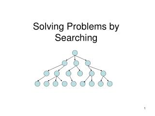
Tree search algorithms • The possible action sequences starting at the initial state form a search tree • Basic idea: • offline, simulated exploration of state space by generating successors of already-explored states (a.k.a.~expanding states)
Implementation: states vs. nodes • A state is a (representation of) a physical configuration • A node is a data structure constituting part of a search tree includes state, parent node, action, path costg(x), depth • The Expand function creates new nodes, filling in the various fields and using the SuccessorFn of the problem to create the corresponding states.
Implementation: general tree search • Fringe (Frontier): the collection of nodes that have been generated but not yet been expanded • Each element of a fringe is a leaf node, a node with no successors • Search strategy: a function that selects the next node to be expanded from fringe • We assume that the collection of nodes is implemented as a queue
Search strategies • A search strategy is defined by picking the order of node expansion • Strategies are evaluated along the following dimensions: • completeness: does it always find a solution if one exists? • time complexity: how long does it take to find the solution? • space complexity: maximum number of nodes in memory • optimality: does it always find a least-cost solution? • Time and space complexity are measured in terms of • b: maximum branching factor of the search tree • d: depth of the least-cost solution • m: maximum depth of the state space (may be ∞)
Uninformed search strategies • Uninformed (blind, exhaustive, brute-force) search strategies use only the information available in the problem definition and do not guide the search with any additional information about the problem. • Breadth-first search • Uniform-cost search • Depth-first search • Depth-limited search • Iterative deepening search
Breadth-first search (BFS) • Expand shallowest unexpanded node • Expands search nodes level by level, all nodes at level d are expanded before expanding nodes at level d+1 • Implemented by adding new nodes to the end of the queue (FIFO queue): • GENERAL-SEARCH(problem, ENQUEUE-AT-END) • Since eventually visits every node to a given depth, guaranteed to be complete. • Also optimal provided path cost is a nondecreasing function of the depth of the node (e.g. all operators of equal cost) since nodes explored in depth order.
Properties of breadth-first search • Assume there are an average of bsuccessors to each node, called the branching factor. • Complete?Yes (if b is finite) • Time?1+b+b2+b3+… +bd + b(bd-1) = O(bd+1) • Space?O(bd+1) (keeps every node in memory) • Optimal? Yes (if cost = 1 per step) • Space is the bigger problem (more than time)
Uniform-cost search • Expand least-cost unexpanded node • Like breadth-first except always expand node of least cost instead of least depth (i.e. sort new queue by path cost). • Equivalent to breadth-first if step costs all equal • Do not recognize goal until it is the least cost node on the queue and removed for goal testing. • Guarantees optimality as long as path cost never decreases as a path increases (non-negative operator costs).
Uniform-cost search • Implementation: • fringe = queue ordered by path cost • Complete? Yes, if step cost ≥ ε • Time? # of nodes with g ≤ cost of optimal solution, O(bceiling(C*/ ε)) where C* is the cost of the optimal solution • Space? # of nodes with g ≤ cost of optimal solution, O(bceiling(C*/ ε)) • Optimal? Yes – nodes expanded in increasing order of g(n)
Depth-first search (DFS) • Expand deepest unexpanded node • Always expand node at deepest level of the tree, i.e. one of the most recently generated nodes. When hit a dead-end, backtrack to last choice. • Implementation: LIFO queue, i.e., put new nodes to front of the queue
Properties of depth-first search • Complete? No: fails in infinite-depth spaces, spaces with loops • Modify to avoid repeated states along path complete in finite spaces • Time?O(bm): terrible if m is much larger than d • but if solutions are dense, may be much faster than breadth-first • Space?O(bm), i.e., linear space! • Optimal? No : • Not guaranteed optimal since can find deeper solution before shallower ones explored.
Depth-limited search (DLS) = depth-first search with depth limit l, i.e., nodes at depth l have no successors • Recursive implementation: Problem if l<d is chosen
Iterative deepening search • Number of nodes generated in a depth-limited search to depth d with branching factor b: NDLS = b0 + b1 + b2 + … + bd-2 + bd-1 + bd • Number of nodes generated in an iterative deepening search to depth d with branching factor b: NIDS = (d+1)b0 + d b^1 + (d-1)b^2 + … + 3bd-2 +2bd-1 + 1bd • For b = 10, d = 5, • NDLS = 1 + 10 + 100 + 1,000 + 10,000 + 100,000 = 111,111 • NIDS = 6 + 50 + 400 + 3,000 + 20,000 + 100,000 = 123,456 • Overhead = (123,456 - 111,111)/111,111 = 11%
Properties of iterative deepening search • Complete? Yes • Time?(d+1)b0 + d b1 + (d-1)b2 + … + bd = O(bd) • Space?O(bd) • Optimal? Yes, if step cost = 1
Repeated states • Failure to detect repeated states can turn a linear problem into an exponential one!
Repeated states • Three methods for reducing repeated work in order of effectiveness and computational overhead: • Do not follow self-loops (remove successors back to the same state). • Do no create paths with cycles (remove successors already on the path back to the root). O(d) overhead. • Do not generate any state that was already generated. Requires storing all generated states (O(b) space) and searching them (usually using a hash-table for efficiency).
Heuristic Search • Heuristic or informed search exploits additional knowledge about the problem that helps direct search to more promising paths. • A heuristic function, h(n), provides an estimate of the cost of the path from a given node to the closest goal state. • Must be zero if node represents a goal state. • Example: Straight-line distance from current location to the goal location in a road navigation problem. • Many search problems are NP-complete so in the worst case still have exponential time complexity; however a good heuristic can: • Find a solution for an average problem efficiently. • Find a reasonably good but not optimal solution efficiently.
Best-first search • Idea: use an evaluation functionf(n) for each node • estimate of "desirability" • Expand most desirable unexpanded node Order the nodes in decreasing order of desirability • Special cases: • greedy best-first search • A* search
Greedy best-first search • Evaluation function f(n) = h(n) (heuristic) • = estimate of cost from n to goal • e.g., hSLD(n) = straight-line distance from n to Bucharest • Greedy best-first search expands the node that appears to be closest to goal
Does not find shortest path to goal (through Rimnicu) since it is only focused on the cost remaining rather than the total cost.