Download
1 / 35
360 likes | 640 Views
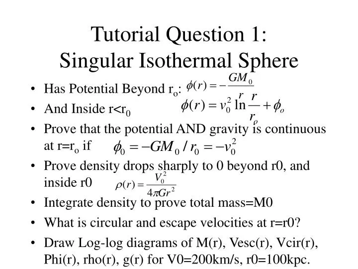
Tutorial Question 1: Singular Isothermal Sphere. Has Potential Beyond r o : And Inside r<r 0 Prove that the potential AND gravity is continuous at r=r o if Prove density drops sharply to 0 beyond r0, and inside r0 Integrate density to prove total mass=M0

E N D
Tutorial Question 1: Singular Isothermal Sphere • Has Potential Beyond ro: • And Inside r<r0 • Prove that the potential AND gravity is continuous at r=ro if • Prove density drops sharply to 0 beyond r0, and inside r0 • Integrate density to prove total mass=M0 • What is circular and escape velocities at r=r0? • Draw Log-log diagrams of M(r), Vesc(r), Vcir(r), Phi(r), rho(r), g(r) for V0=200km/s, r0=100kpc.
Tutorial Question 2: Isochrone Potential • Prove G is approximately 4 x 10⁻³ (km/s)2pc/Msun. • Given an ISOCHRONE POTENTIAL • For M=105 Msun, b=1pc, show the central escape velocity = (GM/b)1/2 ~ 20km/s. • Argue why M must be the total mass. What fraction of the total mass is inside radius r=b=1pc? Calculate the local Vcir(b) and Vesc(b) and acceleration g(b). What is your unit of g? Draw log-log diagram of Vcir(r). • What is the central density in Msun pc-3? Compare with average density inside r=1pc. (Answer in BT, p38)
Example:Single Isothermal Sphere Model • For a SINGLE ISOTHERMAL SPHERE (SIS) the line of sight velocity dispersion is constant. This also results in the circular velocity being constant (proof later). • The potential and density are given by:
Proof: Density Log() r-2 n=-2 Log(r)
Proof: Potential We redefine the zero of potential If the SIS extends to a radius ro then the mass and density distribution look like this: M r ro r ro
Beyond ro: • We choose the constant so that the potential is continuous at r=ro. r r-1 logarithmic
Tutorial Question 3: Show in Isochrone potential • radial period depends on E, not L • Argue , but for • this occurs for large r, almost Kepler
Tidal Stripping • TIDAL RADIUS:Radius within which a particle is bound to the satellite rather than the host system. • Consider a satellite of mass Ms inside radius R is moving in a spherical potential (r) made from a point mass M. R r M(r)
The condition for a particle to be bound to the satellite rather than the host system is: Differential (tidal) force on the particle due to the host galaxy Force on particle due to satellite
Generally, fudge factor k=14, bigger for radial orbits, bigger for point-like mass. • Therefore Tidal Radius is (ambiguously defined as): • The tidal radius is smallest at pericentre where r is smallest. Often tidal radius is only defined when r(t)=pericentre rp. • As a satellite losses mass, its tidal radius shrinks.
The meaning of tidal radius • The inequality can be written in terms of the mean densities. • The less dense part of the satellite is torn out of the system, into tidal tails.
Size and Density of a BH • A black hole has a finite (schwarzschild) radius Rbh=2 G Mbh/c2 ~ 2au (Mbh/108Msun) • verify this! What is the mass of 1cm BH? • A BH has a density (3/4Pi) Mbh/Rbh3, hence smallest holes are densest. • Compare density of 108Msun BH with Sun (or water) and a giant star (10Rsun).
Growth of a BH by capturing objects in its Loss Cone • A small BH on orbit with pericentre rp<Rbh is lost (as a whole) in the bigger BH. • The final process is at relativistic speed. Newtonian theory is not adequate • (Nearly radial) orbits with angular momentum J<Jlc =2*c*Rbh =4GMbh/c enters `loss cone` (lc) • When two BHs merger, the new BH has a mass somewhat less than the sum, due to gravitational radiation.
Tidal disruption near giant BH • A giant star has low density than the giant BH, is tidally disrupted first. • The disruption happens at radius rdis > Rbh , Mbh/rdis3 ~ M* /R*3 • Giant star is shreded. • Part of the tidal tail feeds into the BH, part goes out.
Adiabatic Compression due to growing BH • A star circulating a BH at radius r has • a velocity v=(GMbh/r)1/2, • an angular momentum J = r v =(GMbh r)1/2, • As BH grows, Potential and Orbital Energy E changes (t) • But J conserved (no torque!), still circular! • So Ji = (GMi ri)1/2 =Jf =(GMf rf )1/2 • Shrink rf/ri = Mi/Mf < 1, orbit compressed!
Adiabatic Invariance • Suppose we have a sequence of potentials p(|r|) that depends continuously on the parameter P(t). • P(t) varies slowly with time. • For each fixed P we would assume that the orbits supported by p(r) are regular and thus phase space is filled by arrays of nested tori on which phase points of individual stars move. • Suppose
Initial Final • The orbit energy of a test particle will change. • Suppose • The angular momentum J is still conserved because rF=0.
In general, two stellar phase points that started out on the same torus will move onto two different tori. • However, if potential is changed very slowly compared to all characteristic times associated with the motion on each torus, all phase points that are initially on a given torus will be equally affected by the variation in Potential • Any two stars that are on a common orbit will still be on a common orbit after the variation in Pot is complete. This is ADIABATIC INVARIANCE.
8th Lec • Phase Space
Stellar interactions • When are interactions important? • Consider a system of N stars of mass m • evaluate deflection of star as it crosses system • consider en encounter with star of mass m at a distance b: X=vt v q b r Fperp
Stellar interactions cont. • the change in the velocity Dvperp is then • using s = vt / b • Or using impulse approximation: • where gperp is the force at closest approach and • the duration of the interaction can be estimated as : Dt = 2 b / v
Number of encounters with impact parameter b - b + Db b • let system diameter be: 2R • Star surface density ~ N/R2/Pi • the number encountering • each encounter has effect Dvperp but each one randomly oriented • sum is zero: b+Db
change in kinetic energy • but suming over squares (Dvperp2) is > 0 • hence • now consider encounters over all b • then • but @ b=0, 1/b is infinte! • need to replace lower limit with some bmin • expected distance of closest R/N
Relaxation time • hence v2 changes by Dv2 each time it crosses the system where Dv2 is: Orbit deflected when v2 ~ Dv2 • after nrelax times across the system and thus the relaxation time is:
Relaxation time cont. • collisionless approx. only for t < trelax ! • mass segregation occurs on relaxation timescale • also referred to as equipartition • where kinetic energy is mass independent • Hence the massive stars, with lower specific energy sink to the centre of the gravitational potential.
globular cluster, N=105, R=10 pc • tcross ~ 2 R / v ~ 105 years • trelax ~ 108 years << age of cluster: relaxed • galaxy, N=1011, R=15 kpc • tcross ~ 108 years • trelax ~ 1015 years >> age of galaxy: collisionless • cluster of galaxie: trelax ~ age
Dynamical Friction • DYNAMICAL FRICTION slows a satellite on its orbit causing it to spiral towards the centre of the parent galaxy. • As the satellite moves through a sea of stars I.e. the individual stars in the parent galaxy the satellites gravity alters the trajectory of the stars, building up a slight density enhancement of stars behind the satellite • The gravity from the wake pulls backwards on the satellites motion, slowing it down a little
The satellite loses angular momentum and slowly spirals inwards. • This effect is referred to as “dynamical friction” because it acts like a frictional or viscous force, but it’s pure gravity.
More massive satellites feel a greater friction since they can alter trajectories more and build up a more massive wake behind them. • Dynamical friction is stronger in higher density regions since there are more stars to contribute to the wake so the wake is more massive. • For low v the dynamical friction increases as v increases since the build up of a wake depends on the speed of the satellite being large enough so that it can scatter stars preferentially behind it (if it’s not moving, it scatters as many stars in front as it does behind). • However, at high speeds the frictional force v-2, since the ability to scatter drops as the velocity increases. • Note: both stars and dark matter contribute to dynamical friction
The dynamical friction acting on a satellite of mass Mmoving at vs kms-1 in a sea of particles of density mXn(r) with gaussian velocity distribution • Only stars moving slower than M contribute to the force. This is usually called the Chandrasekhar Dynamical Friction Formula.
For an isotropic distribution of stellar velocities this is: • For a sufficiently large vM, the integral converges to a definite limit and the frictional force therefore falls like vM-2. • For sufficiently small vM we may replace f(vM) by f(0) , define friction timescale by:
Friction & tide: effects on satellite orbit • When there is dynamical friction there is a drag force which dissipates angular momentum. The decay is faster at pericentre resulting in the staircase-like decline of J(t). • As the satellite moves inward the tidal force becomes greater so the tidal radius decreases and the mass will decay.
1st Tutorial g M 2 vesc (E) (r) (r)