Download
1 / 30
300 likes | 304 Views
Space-Filling Curve High-Impedance Ground Planes. b96901128 王郁翔. Outline. 1. Space-Filling Curve 2. Resonance Property 3. High-Impedance Surfaces. Outline. 4. Applications Thin Absorbing Screens Antenna Application DNG bulk media 5. Conclusions. Space-Filling Curve.

E N D
Space-Filling Curve High-Impedance Ground Planes b96901128 王郁翔
Outline • 1. Space-Filling Curve • 2. Resonance Property • 3. High-Impedance Surfaces
Outline • 4. Applications Thin Absorbing Screens Antenna Application DNG bulk media • 5.Conclusions
Space-Filling Curve • A problem in mathematical analysis. • Continuous mapping from line to plane for infinite iteration order.
Why use space-filling curve? • This resonance structure is compacted within a small footprint.(microminiaturization) • The 2D structure is easy to fabricate.
Resonances Simulation • Use method-of-moments(MoM) code to simulate. • Footprint = 30mm*30mm
Resonance Property • The footprint is electrically small. However, the bandwidth is narrow.
High Impedance Surfaces • Reflection coefficient about +1 • Artificial magnetic conductor • Utilizing resonance inclusions on a nonconducting host substrate layer in parallel with a conducting ground plane.
Simulation of Peano Surface • Periodic MoM code • Measure reflection coefficient to frequency. • Condition: Normal incident plane wave. Infinite extent of ground plane and Peano surface of order 2. Perfect metal and dielectric(air).
Simulation of Peano Surface Wire width = 0.5mm footprint = 30mm*30mm distance from ground = 15mm separation = 3.75mm
Simulation of Peano Surface • Footprint and height are relatively small compare to wavelength.(0.153,0.063)(0.076,0.031) • Bandwidth: ±90°
Simulation of Peano Surface • Change height and separation. • y-polarized is less pronounced.
Simulation of Hilbert Surface • Hilbert curve of order 3. Footprint = 30mm*30mm Separation = 4.285mm Height = 15mm • Incident angle from 0 to 60.
Experiment Results • Fabricate curve on 1.575-mm FR-4 substrate with dielectric constant 4.4 and loss tangent 0.02. • Scaled to match the frequency of WR-430 waveguide.(1.7~2.6 GHz)
Experiment Results • Simulate by finite-element method and the measure data.
Varying Loss Tangent • MoM-based IE3D simulation on Peano of order 2 and Hilbert of order 3 for x-polarized wave.
Thin Absorbing Screens • Frequency-selective surfaces. • Thin absorber, application in absorbing material and low observables. • Much smaller than Salisbury screen.
Antenna Application • Put a small dipole antenna above Hilbert surface. • Image current enhanced radiation. • High-performance, low-profile, conformal, flush-mounted antenna.
Antenna Simulation • MoM software package IE3D and NEC-4 based Code GNEC. • Simulate impedance to frequency. • Additional height 15mm 11*11 Hilbert curves copper with conductivity 5.813*107S/m
Efficiency and Directivity • IE3D simulation code
DNG Bulk Media • Embedding many identical space-filling curve inclusions within a host medium. • Simulate electric and magnetic dipole moments to frequency, then use the Maxwell-Garnett mixing formula to analyze this polarizability tensor to obtain effective permittivity and permeability.
Permittivity and Permeability • MoM based code. y-polarized Hilbert curve of order 3 wire radius = 0.125mm
SNG media by Peano • Peano curve inclusions also has negative permittivity and permeability, but in different frequency. • Multifunction media
Conclusions • There are two main problems have to solve. • 1.narrow bandwidth • 2.dependence of the response of space-filling curve on the polarization.