Download
1 / 56
560 likes | 567 Views
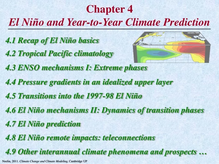
This chapter provides a recap of El Niño basics, explores the tropical Pacific climatology, discusses ENSO mechanisms, prediction methods, and remote impacts. It also covers other interannual climate phenomena and prospects.

E N D
Chapter 4El Niño and Year-to-Year Climate Prediction 4.1 Recap of El Niño basics 4.2 Tropical Pacific climatology 4.3 ENSO mechanisms I: Extreme phases 4.4 Pressure gradients in an idealized upper layer 4.5 Transitions into the 1997-98 El Niño 4.6 El Niño mechanisms II: Dynamics of transition phases 4.7 El Niño prediction 4.8 El Niño remote impacts: teleconnections 4.9 Other interannual climate phenomena and prospects … Neelin, 2011. Climate Change and Climate Modeling, Cambridge UP
4.1 Recap of El Niño basics Supplementary Fig.: Reynolds SST data set [From chapter 1] Climatology 1982-2001 (C) Sea Surface Temp. Dec. 1997 Anomaly (Dec.97 SST-Clim.) Neelin, 2011. Climate Change and Climate Modeling, Cambridge UP
December 1997 Anomalies of precipitationduring the fully developed warm phase of ENSO Recap Figure 1.8 Neelin, 2011. Climate Change and Climate Modeling, Cambridge UP
DJF Low-level wind anomalies during the 1997-98 El Niñorelative to the 1958-98 climatology RecapFigure 1.9 Neelin, 2011. Climate Change and Climate Modeling, Cambridge UP
December 1997 Anomalies of sea level heightduring the fully developed warm phase of ENSO RecapFigure 1.10 Neelin, 2011. Climate Change and Climate Modeling, Cambridge UP
4.2 Tropical Pacific climatology Recap Figure 2.16 Sea surface temperature climatology - January Sea surface temperature climatology - July Neelin, 2011. Climate Change and Climate Modeling, Cambridge UP
RecapFigure 2.13 Precipitationclimatology - January Precipitationclimatology - July Neelin, 2011. Climate Change and Climate Modeling, Cambridge UP
Equatorial Walker circulation Recap Figure 2.14 Adapted from Madden and Julian, 1972, J. Atmos. Sci., and Webster, 1983, Large-Scale Dynamical Processes in the Atmosphere Neelin, 2011. Climate Change and Climate Modeling, Cambridge UP
Pacific in three-dimensions under "Normal" conditions 10 km 15000 km ~28 C ~24 C ~20 C 15 C or colder Figure 4.1 • Atmosphere: • Trade winds blow across Pacific air rises in convergence zone over the warm SSTs in the west. • Ocean: • Thermocline ~100m deeper in west [sea level 40cm higher; see 4.4] • Pressure gradient in ocn. (eastward) balances wind stress in vert avg Neelin, 2011. Climate Change and Climate Modeling, Cambridge UP
Pacific in three-dimensions under "Normal" conditions Figure 4.1 • Recall equatorial upwelling: wind stress & Coriolis force either side of equator give surface divergence • Shallow thermocline in east upwelling brings up colder water • [Equatorial undercurrent above thermocline flows eastward] Neelin, 2011. Climate Change and Climate Modeling, Cambridge UP
4.3 ENSO mechanisms I: Extreme phases Pacific basin under El Niño conditions Figure 4.2a • Warmer SST in east; rainfall tends to spread east • Trade winds weaken • Unbalanced eastward PGF in ocean anomalous currents (in vert • avg through layer above thermocline) thermocline deepens in east • Upwelling brings up water less cold than normal Neelin, 2011. Climate Change and Climate Modeling, Cambridge UP
Pacific basin under La Niña conditions Figure 4.2b • Cooler SST in east; rainfall concentrated in west • Trade winds strengthen • Westward wind stress exceeds eastward PGF in ocean • anomalous currents along Eq. thermocline shallows in east • Upwelling brings up water colder than normal Neelin, 2011. Climate Change and Climate Modeling, Cambridge UP
"It is the gradient of SST along the equator which is the cause of [...] the Walker circulation. An increase in equatorial easterly winds [is associated with] an increase in upwelling and an increase in the east-west temperature contrast that is the cause of the Walker circulation in the first place. [...] On the other hand, a case can also be made for a trend of decreasing speed [...] There is thus ample reason for a never-ending succession of alternating trends by air-sea interaction in the equatorial belt, but just how the turnabout between trends takes place is not yet clear.” 1969 Jakob Bjerknes Neelin, 2011. Climate Change and Climate Modeling, Cambridge UP
The Bjerknes feedbacks (warm phase) Figure 4.3 • Positive feedback loop reinforces initial anomaly Neelin, 2011. Climate Change and Climate Modeling, Cambridge UP
The Bjerknes feedbacks (cold phase) Figure 4.3 [Supplemental] • Positive feedback loop reinforces initial anomaly Neelin, 2011. Climate Change and Climate Modeling, Cambridge UP
The El Niño Pumpkin Neelin, 2011.
4.4 Pressure gradients in an idealized upper layer Idealized upper ocean layer Figure 4.4 • Pressure mass above • At A ocean surface high so PGF from A toward B in upper ocean • Deeperthermocline balances highersea surface PGF small below thermocline • Sea surface height thermocline depth [cm vs. m] Neelin, 2011. Climate Change and Climate Modeling, Cambridge UP
Two positions of the thermocline, indicatingregion of thermocline anomalies Figure 4.5 Neelin, 2011. Climate Change and Climate Modeling, Cambridge UP
4.5 Transitions into the 1997-98 El Niño Buoy from the TAO array Figure 4.6 Courtesy of the Pacific Marine Environmental Laboratory Neelin, 2011. Climate Change and Climate Modeling, Cambridge UP
Global tropical moored buoy array (the original TAO array in the Pacific augmented by subsequent programs) Figure 4.7 Neelin, 2011. Climate Change and Climate Modeling, Cambridge UP
The transition into the 1997-98 El Niño warm phase (Jan. 1997) Figure 4.8 After figures courtesy of David Pierce, Scripps Institute of Oceanography. Neelin, 2011. Climate Change and Climate Modeling, Cambridge UP
The transition into the 1997-98 El Niño warm phase (Apr. 1997) Figure 4.8 cont. After figures courtesy of David Pierce, Scripps Institute of Oceanography. Neelin, 2011. Climate Change and Climate Modeling, Cambridge UP
The transition into the 1997-98 El Niño warm phase (Sep. 1997) Figure 4.8 cont. After figures courtesy of David Pierce, Scripps Institute of Oceanography. Neelin, 2011. Climate Change and Climate Modeling, Cambridge UP
The transition into the 1997-98 El Niño warm phase (Jan. 1998) Figure 4.8 cont. After figures courtesy of David Pierce, Scripps Institute of Oceanography. Neelin, 2011. Climate Change and Climate Modeling, Cambridge UP
The transition into the 1998-98 La Niña cold phase (May 1998) Figure 4.9 After figures courtesy of David Pierce, Scripps Institute of Oceanography. Neelin, 2011. Climate Change and Climate Modeling, Cambridge UP
The transition into the 1998-98 La Niña warm phase (Sep. 1998) Figure 4.9 cont. After figures courtesy of David Pierce, Scripps Institute of Oceanography. Neelin, 2011. Climate Change and Climate Modeling, Cambridge UP
The transition into the 1998-98 La Niña phase (Jan. 1999) Figure 4.9 cont. After figures courtesy of David Pierce, Scripps Institute of Oceanography. Neelin, 2011. Climate Change and Climate Modeling, Cambridge UP
4.6 El Niño mechanisms II: Dynamics of transition phases Schematic of an equatorial jet Figure 4.10 • deep thermocline = high pressure in upper ocean, H • current can flow along Eq. (Coriolis=0) • equatorial jet: balance of deep thermocline and current anomalies near equator (with PGF= Coriolis; note change in CF with latitude crucial) Neelin, 2011. Climate Change and Climate Modeling, Cambridge UP
Schematic of an equatorial jet showing that it canextend itself eastward but not westward Figure 4.11 Neelin, 2011. Climate Change and Climate Modeling, Cambridge UP
Currents carry mass affects pressure • Deep thermocline extends eastward where mass added (edge moving eastward = “Kelvin wave”) • NB: something has to continually supply mass in the west for the jet to persist • Shallow thermocline and westward currents also give equatorial jet( just switch sign of anoms) • Low is extended by removing water ( in the ocean upper layer), so also extends eastward Neelin, 2011. Climate Change and Climate Modeling, Cambridge UP
Kelvin wave front at the eastern edge of an equatorial jet Figure 4.12 Neelin, 2011. Climate Change and Climate Modeling, Cambridge UP
Response of the ocean to a westerly wind anomaly Re: onset and demise of El Niño warm phase Figure 4.13 • To east of the wind anomalies, equatorial jet (Kelvin wave) extends east, deepening thermocline (H) • (recall: warms SST…) • To west, inflow of water to jet (in oc. upper layer) comes from off the equator (but little effect on SST) • shallow thermocline in west extends westward (Rossby wave), as mass transferred to east by jet • when reaches western boundary, can no longer supply mass by extending shallow region • Weakening of jet extends eastward, ending warm phase • As wind anomalies weaken, shallow thermocline extends eastward: transition to cold phase Wind anoms currents Deep Thermocline anoms Neelin, 2011. Climate Change and Climate Modeling, Cambridge UP
Response of the ocean to a easterly wind anomaly Re: Onset and demise of La Niña cold phase (supplementary Fig.) • Same as Figure 4.13 but anomalies of opposite sign Neelin, 2011. Climate Change and Climate Modeling, Cambridge UP
Meantime, in the West Pacific (subsurface) ENSO transitions Recall:feedbacks that strengthen El Niño Delay: no surface effect until… And vice versa… Onset of La Niña cold phase Figure 4.14 Neelin, 2011. Climate Change and Climate Modeling, Cambridge UP
4.7 El Niño prediction Forecast of SST anomalies (as three month averages) • Forecast of the onset of the 1997-98 El Niño • From National Center for Environmental Prediction climate model • Data through March 1997 (previous wind stress anomalies, ocean subsurface temperatures, SSTs,…) • [“Data assimilation” process includes interpolation of sparse observations to all model grid points, balancing terms in model equations,…] • climate model runs forward in prediction mode (from April) Figure 4.15 Courtesy of the National Center for Environmental Prediction Neelin, 2011. Climate Change and Climate Modeling, Cambridge UP
Supplementary Figure: NCEP Forecast vs. Observation Courtesy of the National Center for Environmental Prediction Neelin, 2011. Climate Change and Climate Modeling, Cambridge UP
Commonly used index regions for ENSO SST anomalies Recall: Figure 1.5 Neelin, 2011. Climate Change and Climate Modeling, Cambridge UP
Series of forecasts of SST anomalies averagedover the Niño-3 region of the equatorial Pacific Figure 4.16 • Track record of forecasts: • From forecasts made each month, collect all the forecast SST anomalies at 3-month lead (i.e. after each forecast had gone three months into the future), 6-month lead, 9-month lead, … • E.g. March 1997 forecast shown • Compare each forecast to the SST anomaly that was later observed (solid line) • skill decreases with longer lead; still useful at 9 months Courtesy of the National Center for Environmental Prediction Neelin, 2011. Climate Change and Climate Modeling, Cambridge UP
Loss of skill in ENSO forecasts: Imperfections in the forecast system -e.g., model errors, scarcity of input data (can be improved, if $) Fundamental limits to predictability -weather unpredictable beyond two weeks (chaos theory): slightly different initial conditions lead to later weather patterns as dissimilar as weather maps chosen at random (except for aspects determined by sea surface temperature…) - “weather noise”:acts like a random forcing on slow ocean-atmosphere interaction e.g. in the Bjerknes hypothesis, SST gradient determines average strength of Tradewinds. But in a particular month, storms or other transient weather events can cause equatorial Easterlies to differ from this, causing a greater or lesser change of currents than you would expect from the SST anomalies 4.7.1 Limits to skill in ENSO forecasts Neelin, 2011. Climate Change and Climate Modeling, Cambridge UP
Effects of weather noise on the ENSO cycle Figure 4.17 • Schematically, random weather events cause cycle to depart from the evolution it would otherwise have had • Cumulative effects cause departure from prediction Neelin, 2011. Climate Change and Climate Modeling, Cambridge UP
An ensemble of forecasts duringthe onset of the 1998-99 La Niña • Start coupled model from different ocean initial conditions (leading also to changes in atm. ) • Initial differences grow Þ ensemble of prediction runs • Ensemble spread gives estimate of uncertainty • Spread tends to grow with time (due to weather noise & coupled feedbacks) • Ensemble mean gives best estimate Figure 4.18 Courtesy of the European Centre for Medium-range Weather Forecasting. Neelin, 2011. Climate Change and Climate Modeling, Cambridge UP
Supplementary Figure ECMWF forecast of the 09/10 El Nino from May 2009 with overlaid observations Courtesy of the European Centre for Medium-range Weather Forecasting. Neelin, 2011. Climate Change and Climate Modeling, Cambridge UP
Supplementary Figure ECMWF forecast from March 2010 predicting transition to La Niña of 2010 Courtesy of the European Centre for Medium-range Weather Forecasting. Courtesy of the European Centre for Medium-range Weather Forecasting. Neelin, 2011. Climate Change and Climate Modeling, Cambridge UP
Supplementary Figure ECMWF forecast from March 2010: with overlaid observations for verification Courtesy of the European Centre for Medium-range Weather Forecasting. Courtesy of the European Centre for Medium-range Weather Forecasting. Neelin, 2011. Climate Change and Climate Modeling, Cambridge UP
Supplementary Figure ECMWF forecast from Sept. 2010: with overlaid observations for verification Courtesy of the European Centre for Medium-range Weather Forecasting. Courtesy of the European Centre for Medium-range Weather Forecasting. Neelin, 2011. Climate Change and Climate Modeling, Cambridge UP
Supplementary Figure ECMWF forecast from March 2011 Courtesy of the European Centre for Medium-range Weather Forecasting. Courtesy of the European Centre for Medium-range Weather Forecasting. Neelin, 2011. Climate Change and Climate Modeling, Cambridge UP
4.8 El Niño remote impacts: teleconnections Regions with statistically reliable relation of precipitation andsurface air temperature to El Niño and La Niña Figure 4.19 • Impact regions change with seasonal climatology • La Niña similar but opposite sign Neelin, 2011. Climate Change and Climate Modeling, Cambridge UP
Patterns of typical response to El Niño observedfor northern hemisphere winter Figure 4.20 Neelin, 2011. Climate Change and Climate Modeling, Cambridge UP
Jet stream and storm track changesassociated with El Niño or La Niña Figure 4.21 Neelin, 2011. Climate Change and Climate Modeling, Cambridge UP
Schematic of shift of probability distribution of precipitation, e.g. in Southern California, during El Niño • E.g., find value of precip which only 1/3 of winters exceed, and ask what fraction of El Niño winters exceed it • Probability of rainy winter enhanced (but far from certain) Figure 4.22 Neelin, 2011. Climate Change and Climate Modeling, Cambridge UP