Download
1 / 28
280 likes | 301 Views
This lecture discusses the use of nonlinear equation solvers, such as the successive substitution and Newton-Raphson methods, in solving steady-state and unsteady-state problems. It also introduces control systems and their application in advanced air systems. Topics covered include under-relaxation, over-relaxation, and the PID control algorithm.

E N D
Lecture Objectives: • Discuss HW4 • Nonlinear equation solvers • Continue with advance air systems • Introduce control systems
Successive substitution method • Iterative method: • Requires initial guess • Requires equation in explicit form • Can be used for solution of - steady-sate or • - unsteady-state problems • For unsteady-state problem we have to iterations for each time step Solution for one time step: Simple Example: X-Y/2=-1 X2-Y=-3 X, Y are any physical variables We know the solution: By substitution method we get: X2-2x+1=0 → X=1, Y=4 Explicit form: X=Y/2-1 Y=X2+3
Successive substitution method Simple Example: Explicit form: X=Y/2-1 Y=X2+3 Initial guess ? End of iteration ? X=Y/2-1 Y=X2+3 Y=… X=… yes Y=2 no Solution: Solution for One time step
RY n n-1 Successive substitution method When to stop with iterations? We DO NOT know the exact solution! Residual: Difference in result between two iterations RY=|Y(n)-Y(n-1)|<e , e is defined by requested accuracy • For example: eY=0.0004 • Iteration 99 Y(99) =3.96132 • Iteration 100 Y(100)=3.96169 |Y(100)-Y(99)|=0.00037<eY • stop the iterations
Iterative method Relaxation with iterative solvers: When the equations are highly nonlinear it can happen that you get divergency in iterative procedure for solving considered time step divergence variable solution convergence Solution is Under-Relaxation: Y*=f·Y(n)+(1-f)·Y(n-1) Y – considered parameter , n –iteration , f – relaxation factor For our example Y*in iteration101=f·Y(100)+(1-f) ·Y(99) f = [0-1] – under-relaxation -stabilize the iteration f = [1-2] – over-relaxation - speed-up the convergence iteration Value which is should be used for the next iteration Under-Relaxation is often required when you have nonlinear equations!
Newton-Raphson method • Considerably better method than • Successive substitution method • Faster convergence • Used in many professional tools (MathCAD, EES, MatLab, Mathematica, etc) • More complex for programming • Requires linear solver • Based on Taylor-Series Expansion • You need first derivative for each function to create the Jacobean matrix • Equations in the form where all side are on one side of equality sign Our simple example: X-Y/2=-1 → X-Y/2+1=0 X2-Y=-3 → X2-Y+3=0
Function values for guessed variables Jacobean matrix Unknowns (correction Dxi) Newton-Raphson method(this is used in most equation solvers) Section 6.11 of handouts Our simple example: f1 = X-Y/2+1=0 f2 = X2-Y+3=0 Steps: 0) Find derivatives d(f1)/dX =1 , d(f1)/dY =-1/2 d(f2)/dX =2X , d(f2)/dY =-1 1) Initial guess: Y(0)=2, X(0)=2 2) Find f1(Y(0),X(0))=2-2/2+1=2 f2(Y(0),X(0))=22-2+3=5 3) Using derivatives and guess values find the Jacobean matrix 4) Solve the matrix using linear solver and find DX and DY 5) Find Y(1)=Y(0)+ DY, X(1)=X(0)+ DX, Repeat step (2) with Y(1) and X(1) ….. Follow the procedure till convergence
Various Desiccant Systems D. La, Y.J. Dai *, Y. Li, R.Z. Wang, T.S. Ge Technical development ofrotary desiccant dehumidification and air conditioning: A review” Renewable and Sustainable Energy Reviews http://ac.els-cdn.com/S1364032109001737/1-s2.0-S1364032109001737-main.pdf?_tid=4e770220-bb3b-11e3-a8b2-00000aacb361&acdnat=1396535094_db711889daf20a355a7da4e49f4a3ab6
The PID control algorithm For our example of heating coil: constants time e(t) – difference between set point and measured value Position (x) Differential Proportional Integral Differential (how fast) Proportional (how much) Integral (for how long) Position of the valve
Proportional Controllers x is controller output A is controller output with no error (often A=0) Kis proportional gain constant e = is error (offset)
Unstable system Stable system
Issues with P Controllers • Always have an offset • But, require less tuning than other controllers • Very appropriate for things that change slowly • i.e. building internal temperature
Proportional + Integral (PI) • K/Ti is integral gain If controller is tuned properly, offset is reduced to zero Figure 2-18a
Issues with PI Controllers • Scheduling issues • Require more tuning than for P • But, no offset
Proportional + Integral + Derivative (PID) • Improvement over PI because of faster response and less deviation from offset • Increases rate of error correction as errors get larger • But • HVAC controlled devices are too slow responding • Requires setting three different gains
The control in HVAC system – only PI Proportional Integral value Set point Proportional affect the slope Integral affect the shape after the first “bump” Set point
The Real World • 50% of US buildings have control problems • 90% tuning and optimization • 10% faults • 25% energy savings from correcting control problems • Commissioning is critically important
HVAC Control Example : Dew point control (Relative Humidity control) fresh air damper filter cooling coil heating coil filter fan mixing T & RH sensors Heat gains Humidity generation We should supply air with lower humidity ratio (w) and lower temperature We either measure Dew Point directly or T & RH sensors substitute dew point sensor
Relative humidity control by cooling coil Cooling Coil Mixture Room Supply TDP Heating coil
Relative humidity control by cooling coil (CC) • Cooling coil is controlled by TDP set-point if TDP measured > TDP set-point → send the signal to open more the CC valve if TDP measured < TDP set-point → send the signal to close more the CC valve • Heating coil is controlled by Tair set-point if Tair < Tair set-point → send the signal to open more the heating coil valve if Tair > Tair set-point → send the signal to close more the heating coil valve Control valves Fresh air mixing cooling coil heating coil Tair & TDP sensors
Mixture 3 DPTSP Set Point (SP) Mixture 2 Mixture 1 DBTSP Sequence of operation(PRC research facility) Control logic: Mixture in zone 1: IF (( TM<TSP) & (DPTM<DPTSP) ) heating and humidifying Heater control: IF (TSP>TSA) increase heating or IF (TSP<TSA) decrease heating Humidifier: IF (DPTSP>DPTSA) increase humidifying or IF (DPTSP<DPTSA) decrease humid. Mixture in zone 2: IF ((TM>TSP) & (DPTM<DPTSP) ) cooling and humidifying Cool. coil cont.: IF (TSP<TSA) increase cooling or IF (TSP>TSA) decrease cooling Humidifier: IF (DPTSP>DPTSA) increase humidifying or IF (DPTSP<DPTSA) decrease hum. Mixture in zone 3: IF ((DPTM>DPTSP) ) cooling/dehumidifying and reheatin Cool. coil cont.: IF (DPTSP>DPTSA) increase cooling or IF (DPTSP<DPTSA) decrease cooling Heater control: IF (TSP>TSA) increase heating or IF (TSP<TSA) decrease heating