Download
1 / 42
420 likes | 528 Views
This document provides a comprehensive overview of data processing methodologies in solar observations, detailing the various data levels, their advantages, and limitations. It addresses common issues encountered during data processing, such as channel geometry errors, spatially distorted results due to scanning problems, and interference from clouds. The guide also presents solutions for enhancing telescope pointing in X-scans and improving signal-to-noise ratios. Detailed procedures are provided to correct periodic fluctuations in results and optimize data retrieval and analysis through different stages of processing.

E N D
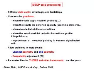
MSDP data processing • Different data levels: advantages and limitations • How to solve problems: • when the code stops (channel geometry…) • when the results are distorted spatially (scanning problems…) • when clouds disturb the observations • when the results exhibit periodic fluctuations (profile interpolations) • improvement of telescope pointing in X-scans, signal/noise ratio. … • A few problems in more details: • Channelgeometry andgrid geometry • Cospatiality adjustment (2D) • - Parameter files for THEMIS and other instruments over the years Pierre Mein, MSDP whorkshop, Tarbes 2006
THEMIS / MSDP Different data levels • Raw data fits 3 files t… • 1)sequence.par + msdpauto (idl) • 1 file for 1 window and 1 time fits 1 files b…… • creates new directory + ms.par • 2)new directory+ ms.par + ms1 (f90) • a)Calibrations (geometry, photometry) • Superposable calibrated channels msdp files c…. • b)Results with preliminary wavelength calibration • Bisector for each observing time msdp msdp files d…. • Bisector for full scan msdp files q…. • c) Results with internal wavelength calibration • Line profiles for each time msdp files r…. • Line profiles for full scan msdp files p….
Raw data • Simultaneous 2D spectro-polarimetry • - Example of 16 channels (alternate wavelengths) • Grid at first focus in front of polarization analyser Focus Sp1 Focus Sp2 Focus F1 I+V I-V
Files t… raw data fits 3 Files b… 1 file for 1 window and 1 time fits 1 t….b…. b….b…. Scan files t….x…. b….x…. Dark current t….y…. b….y…. Flat field t….z…. b….z…. Field stop
Line profile restoration (9 channels, without polar. analysis, VTT)
Superposable calibrated channels files c…. For each time, series of identical rectangles, at different l Might be used for direct line profile inversion to specify parameters of a solar model without profile interpolations This would avoid interpolations and loss of accuracy (see corrections of periodic fluctuations…)
Results for each time Files d… preliminary wavelength calibration (mainly bisector computations) Files r… calibrated wavelengths (mainly line profiles) - In case of series of exposures (bursts), allow seeing effects correction by destretching (Pic du Midi) - Provide the full data for 1 observing time without loss of field-of-view (overlaps mix successive observations in q- and p- files). - Can be used to investigate far line wings near the edges of channels (one wing near one edge)
Full scan results Files q…. (bisector) Not corrected l0 Files p…. (profiles) Corrected l0 • The standard processing provides • Without polarization With Zeeman circular • analysis analysis • Additional arrays • q-files with intensity near line centre Stokes V near line centre • sum of intensities +/- dl Int. differences (cospatiality test) • difference of intensities +/- dl Stokes V at +/- dl • intensity from bisector +/- dl velocity from bisector +/- dl • velocity from bisector +/- dl B// from bisector +/- dl • - p-files with intensity line profile Stokes V line profile In case of Q,U,V observations, separate files for +Q,-Q,+U,-U,+V,-V noted (param nqseul) 1 2 3 4 5 6 and beam-exchange results 7 8 9
How to solve problems 1) If the IDL interface « msdpauto » stops ? (the b- files are not created) -Check the directory name of data in msdpauto, ’…..directory….’ - Check the number bs of channels in « sequence.par » (the code divides the frames in 2 windows of 8 channels in the case of 16 channels beam-shifters)
How to solve problems 2) in all cases when the Fortran code « ms1 » stops ? - The most simple way to modify the parameters of « ms1 » is to edit and modify « ms.par », and to run again « ms1 » - To modify parameters automatically for a full campaign, it is necessary to modify « tyear.par » if the parameters are present in that file (t for Themis,year = 2002, 2003, … « pyear.par » for Pic du Midi, « myear.par » for Meudon,…) In that case, run again the IDL interface « msdpauto »
If the code stops before channel geometry determination ? (before any message including « milgeo ») Either the code does not read files with the good format: Check sundec and iswap in ms.par, or sd in sequence.par Or the code does not find the data files: Check that files y,z are present and also x if parameter idc=1 Check also that the directory name is correct in ms.par
If the code stops and asks for an « increase of milgeo » ? • The code cannot determine the edges of channels. • 1) If the geo.ps file is available • display it by • ggv geo.ps • And modify in ms.par the parameters after headers « bmg » • such as thresholds si,sj,sgi,sgj,… (see param.txt for details)
If the code stops and asks for an « increase of milgeo » ? • 2) If the geo.ps file is not available, • display the average field-stop file by • IDL • image = readmsdp(‘z………’) • tvscl,im • and check the location of channels (parameters i1, i2m), • the sharpness (intvi,intvj)…
How to solve problems if the resulting q- and p-files exhibit strong spatial distortions ? Something is wrong in the parameters specifying symetries and scanning directions, or grid location. - Small rectangles: Some of the following parameters must be modified: inveri, inverj, xfirst Note also that invi, invj determine the final symetries of the maps invern, inverl, invers determine signs and orders of wavelengths and Stokes parameters
Xfirst = 0 Xfirst = 1 Xfirst = 1, norma = 0199 NaD1, intensity +/-40mA, 16 oct 2002
How to solve problems if the resulting q- and p-files exhibit strong spatial distortions ? - Lines parallel to the X-scanning direction: Display grid.ps and modify caldeb,ideb, igri, itgri (see param.txt) Automatic correction with caldeb = 1
How to correct cloud effects ? Intensities disturbed by clouds Velocities and B// not disturbed
Correctionnorma (norma=0289) Intensities corrected
How to solve problems if q- and p-files exhibit spatial periodic fluctuations ? The limited spectral resolution leads to slight periodic errors due to line profile interpolations, which produce kinds of fringes parallel to the longer edge of field-stop. Several ways can be used to correct them.
How to correct grooves due to interpolation between channels ?Themis, 16 channels, without correction I_0 I_120 v_120 B_120
Spatial wavelength P of fluctuations versus y l= L + n Dl + y * (dl/dy) Channel step y P x P= Dl*(dy/dl) Themis: 16 channels P ~ 1.4 arcsec 9 channels P ~ 4.1 arcsec For corrections, we assume that, locally, l does not depend ony (we neglect the inclination and curvature of lines l = ct)
Profile curvature deduced from neighbouring points • curvd= 4 (curvr = 4) I’(3) Z I’ y P/2 I -P/2 I’’ I(3) x I ’’(3) Themis 16 channels0.7 ’’ 9 channels2’’ Interval 4-5: Z = polynomial degree 4 Z(3)=I(3) Z(4)=I(4) Z(5)=I(5) Z(6)=I(6) Z(3.5)+Z(5.5)-2*Z(4.5) = (I’(4)+I’’(3)+I’(6)+I’’(5)-2*(I’(5)+I’’(4)))/2
2) Fourier filtering Crecd (w1d) w2d (w3d) Crecr (w1r) w2r (w3r) 0/1 0/1 0/1 L = 2P P P/2 y P M x j crecd i Correction = - Ct* <<I(x,y)*apod(x)>-crecd,+crecd *cos(2py/L)*apod(y)>-P,+P
Themis, 16 channels, Curvaturecurvd = 4, Fouriercrecd = 2000, w2d = 1 I_0 I_120 v_120 B_120
Corrections without any loss of spatial resolution 1) Power functions I’=(I-Iz)**a a= milalp / 1000 Iz=Imin * milzero / 1000 Interpolation I = Iz + I’**(1/a) 2) l smoothingchannels n-1, n, n+1 weights ¼, ½, ¼ nlisd = 2 nlisr = 2 (effect similar to Fourier filtering w1 = 1(w1r = 1) which degrades slightly the spatial resolution instead of the spectral one)
3) Mean departures between successive scan steps Field of view of a d-file (1 t-value) M y lcrecq x Each quantity (I, v, Stokes..) of all files d (or r) from the same scan defines a function F(x,y,t) 1) Computation of the mean A of F over x,y,t after rejection ( departures > sigma * milsigq /1000 ) 2) For each pixel x,y, computation of the average D(x,y) of departures from A for all times t 3) Smoothing D' of D(x,y) versus x over –L,+L around M (L = lcrecq/ 1000 arcsec) 4) The correction is - D' if crecq = 2 (folding with period P if crecq = 1) The correction depends only on x and y. It does not degrade the spatial resolution.
VTT, 23 oct 2002 Ha without correction I_0 460 * 180 arcsec
Without correction I_290
Without correction v_290
2D correlations and pointing corrections Mean departures quick.ps P
VTT Ha2D Correlations lcorq = 2 icormq = 4000 copasq = 2000 milcoq = 300 ( 2d array) (4’’) (2’’) (0.3) Corrections by mean departures crecq = 2 lcrecq = 10000 milsigq = 2000 (10’’) (2 * s) I_0
v_290 Disc centre
Some additional improvements Signal/noise ratio: can be improved by smoothing versus wavelength nlisd,nlisr versus x ilisdr versus y jlisdr Scattered light rate = scatter /1000 (computed over each line at constant l) Very large scans increase the pixel = milsec /1000 arcsec
Cospatiality adjustment 0.5 arcsec error introduced manually (itana+500) Cospatiality test
Correction calana(calana=1, quadratic interpol.) between dx = +/-1’’ et dy = +/-0.5’’) Cospatiality test
Channel geometry Because of a shift betweenfield-stop and flat-field, due to misadjustment of grating angles, too large to be corrected by the code, the flat-field must be used instead of the field-stop (calfs = -1) But channel edges are more difficult to determine because of the presence of lines in some channels. nleft, nright allow to locate some edges by similarity with neighbouring channels Field stop (8 channels) Flat field
calfs = -1 flat field used as field stop nright = 3 right edge of channel 3deduced from left edge +size of channel 4
Steps Corrections Files Output results b geo flat bmc geom calib Aligned and calibrated channels Possible direct inversion avoiding interpolation corrections c Power fcts Scattered light Normalization Smoothing l Profile curvature Fourier filtering Cospatiality cmd Individual maps I, v, B// Possible destretching d quick 2D - correl Average departures q Large maps I, v, B// Like cmd except cospatiality cmr Individual maps Profiles I, Q, U, V with calibrated central wavelength r Like quick except 2D - correl prof p Large spectrohéliog. I,Q,U,V Inversions with constant l
Parameter files which specify MSDP instruments THEMIS t2000.par, t2001.par,…t2005.par LJR at Pic du Midi p2001.par,p2002.par,…p2005.par Meudon Solar Tower m2003.par,m2004.par,m2005.par processing msdpauto + ms1 VTT/ DALSA cameras example of ms.par processingdalsa +ms1 Wroclaw Large Coronagraph examples ofms.par (?) processing similar to ms1