Download
1 / 1
10 likes | 188 Views
Can wavelet analysis provide an automated technique to create the Dst index? Agnieszka Jach 1 , Piotr Kokoszka 1 , Lie Zhu 2 , Jan Sojka 2 1 Mathematics and Statistics Department, 2 Center for Atmospheric and Space Sciences, Utah State University, Logan, UT. Wavelet-based procedure

E N D
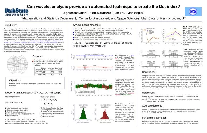
Can wavelet analysis provide an automated technique to create the Dst index? Agnieszka Jach1, Piotr Kokoszka1, Lie Zhu2, Jan Sojka2 1Mathematics and Statistics Department, 2Center for Atmospheric and Space Sciences, Utah State University, Logan, UT • Wavelet-based procedure • Filter out Periodic component from details Dj associated with Sq system, i.e., details at levels j = 8,9,10, corresponding to 8h, 12h and 24h frequencies, respectively • Eliminate Long-term component captured by SJ by replacing SJ with the average of X • Remove Noise via thresholding of the wavelet coefficients Wj at low levels (j = 1,…,7), i.e., those associated with high frequencies • Adjust for the magnetic latitude, and center to remove B • Average four (or three) stations to get wavelet-based index Results – Comparison of Wavelet Index of Storm Activity (WISA) with Kyoto Dst Introduction The primary geomagnetic storm indicator is the Dst index. This index has a well established ‘recipe’ by which ground-based observations are processed to produce this single planetary index. Typically four ground stations are used in this process. Assuming the calibration, data gaps, and measurement uncertainties are known, the major step in creating the Dst is the subtraction of the daily Sq variation. Determining a quiet day Sq variation, which has seasonal dependence as well as shorter term ones, is the ‘art’ in this analysis procedure. Schemes for selecting this can be as quantitative as averaging the three quietest days in the month, i.e., a new Sq variation is inferred each month. The question addressed by this study is whether it is feasible for an automated technique to remove the Sq without operator intervention? Our study is based on wavelet analysis. An algorithm was developed for four ground stations for two months of measurements (March and April 2001). The results of applying the procedure to a year of data and then comparing these with the Kyoto Dst are presented. Additional comparisons with the Kyoto Dst are presented in which the automated analysis uses only three of the four magnetometer data sets. Fig.4. WISA and Dst on March 31 and July 4 from Fig. 1. 95% confidence limits for WISA, were calculated from the increments of WISA. 99% of observations of Dst are within these limits, meaning that the two indices do not differ significantly compared to the hour-to-hour changes. Fig.5. Histograms for the differences between WISA and Dst based on four triplets of Dst stations. The excluded station is indicated by a blank. There is no distinction between disturbed and quiet periods. Bars span 95% of the data, i.e., data within 2 standard deviations of the average. Fig.1. Minute values of WISAand hourly values of Kyoto Dst for the year 2001. By definition, the average of WISA is zero as a result of adding four zero-mean magnetograms. Two days; disturbed, Mar 31, and quiet, July 4, are zoomed in Fig. 4. • Dst index • H component at 4 low-latitude stations, hourly • Quietest days for each month at each station are used to estimate secular and diurnal variations Conclusions Using wavelet-based procedure, we are able to create the storm activity index that is within 10 nT of Kyoto Dst for 2001 without any human input. This procedure also allows us to estimate Sq system by filtering out portions of the wavelet details that contain three different harmonics associated with that system. The procedure is automated and can be applied to two-months’ worth of data or more. By definition, the average of WISA is zero and thus, at this point, we are unable to obtain the reference level. Future work, that is currently underway, is to investigate the removal of magnetic signatures arriving from non-Dst current sources, such as the Birkeland Currents associated with the auroral electrojets. References Sugiura, M. 1964. Hourly values of equatorial Dst for the IGY. Ann. Int. Geophysical Year 35:945. Percival, D. B., Walden, A. T. 2000. Wavelet Methods for Time Series Analysis. Cambridge University Press, Cambridge. Acknowledgments Funding for the WAMI (Wavelet Analysis of Magnetosphere-Ionosphere) project is provided by an NSF grant DMS-0413653. Data is provided by the global network of magnetic observatories, INTERMAGNET. For further information Please contact ajach@cc.usu.edu. PDF and PS versions of the manuscript on which the poster is based are available upon request. Poster is available at http://cc.usu.edu/~ajach. Fig.2. Relative comparison of WISA with Dst. Sixty 1-min observations of WISA were averaged and compared with one 1-h value of Dst. Dst was adjusted by its average, -18 nT, for the year 2001. Differences were divided into two groups, for disturbed periods and quiet periods. Objectives Eliminate human input when creating the storm activity index – automate the procedure. Model for a magnetogram X = [X1,…,XT]’(H comp.) Physical representation B: Internal magnetic field (constant) A: Disturbance due to storm activity P: Periodic (diurnal) component L: Long-term (seasonal or longer) component N: Noise component t: time in minutes, t = 1,…,T = 525600 = 1 year j: level j, corresponds to time scale 2j minutes, j = 1,…,J = 19 Wj are associated with Fourier frequencies in the interval [2-(j+1), 2-j] Wavelet representation Wj: Wavelet coefficients ~ high freq. VJ : Scaling coefficients ~ low freq. Wj : Matrix defining wavelet transform VJ : Matrix defining wavelet transform Dj,: Wavelet details SJ : Wavelet smooths Fig.3. Histograms for the disturbed and quiet differences from Fig.2. Bars span 95% of the data, i.e., data within 2 standard deviations of the average. Both histograms look very normal with standard deviations ~4 nT, even though the indices may be based on different data.