Download
1 / 25
250 likes | 440 Views
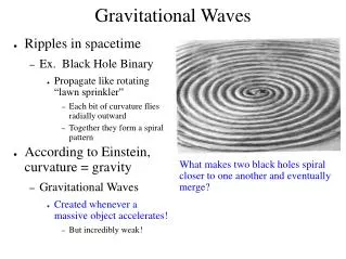
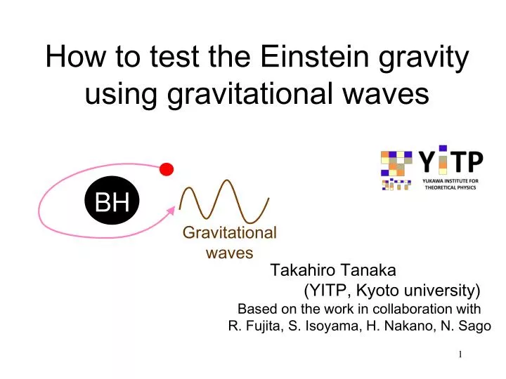
How to test the Einstein gravity using gravitational waves. Gravitational waves. Takahiro Tanaka (YITP, Kyoto university ). Based on the work in collaboration with R. Fujita, S. Isoyama, H. Nakano, N. Sago. Binary coalescence. Clean system. (Cutler et al, PRL 70 2984(1993)).

E N D
How to test the Einstein gravity using gravitational waves Gravitational waves Takahiro Tanaka (YITP, Kyoto university) Based on the work in collaboration with R. Fujita, S. Isoyama, H. Nakano, N. Sago
Binary coalescence Clean system (Cutler et al, PRL 70 2984(1993)) • Inspiral phase (large separation) • Merging phase - numerical relativity • Ringing tail - quasi-normal oscillation of BH Negligible effect of internal structure Accurate prediction of the wave form is requested • for detection • for parameter extraction • for precision test of general relativity (Berti et al, gr-qc/0504017 )
Template (prediction of waveform) 1PN 1.5PN for circular orbit Do we need to predict accurate wave form? • We know how higher expansion goes. ⇒Only for detection, higher order template may not be necessary? • But we need higher order accurate template • for the test of GR.
Propagation of GWs as an example of GR test • Chern-Simons Modified Gravity The evolution of background scalar field q is hard to detect. : J0737-3039(double pulsar) (Yunes & Spergel, arXiv:0810.5541) Right handed and left handed gravitational waves are magnified differently during propagation, depending on the frequencies. • Ghost free bi-gravity Both massive and massless gravitons exist. →n oscillation-like phenomena (in preparation)
Methods to predict wave form Post-Newton approx. ⇔ BH perturbation • Post-Newton approx. • v < c • Black hole perturbation • m1 >>m2 BH pertur- bation Post Teukolsky post-Newton ○ : done Red ○means determination based on balance argument
Extrime Mass Ratio Inspiral(EMRI) • Inspiral of 1~100MsolBH of NS into the super massive BH at galactic center (typically 106Msol) • Very relativistic wave form can be calculated using BH perturbation • Many cycles before the coalescence ~O(M/m) allow us to determine the orbit precisely. • Clean system BH The best place to test GR.
Black hole perturbation • M >>m • v/ccan be O(1) Gravitational waves Linear perturbation :simplemaster equation Regge-Wheeler-Zerilli formalism (Schwarzschild) Teukolsky formalism (Kerr)
Leading order wave form Energy balance argument is sufficient. Wave form for quasi-circular orbits, for example. leading order
Evolution of general orbits If we know four velocity um at each time accurately, we can solve the orbital evolution in principle. On Kerr background there are four “constants of motion” constant in case of no radiation reaction Normalization of four velocity: Energy: Killing vector for time translation sym. Angular momentum: Killing vector for rotational sym. Carter constant: Killing tensor Quadratic and un-related to Killing vector (simple symmetry of the spacetime) One to one correspondence We need to know the secular evolution of E,Lz,Q.
The issue of radiation reaction to Carter constant • E, Lz⇔ Killing vector • Conserved current for the field corresponding • to Killing vectorexists. As a sum conservation law holds. × However, Q⇔ Killing vector • We need to directly evaluate the self-force acting on the particle, but it has never been done for general orbits in Kerr because of its complexity.
§3 Adiabatic approximation for Q which is different from energy balance argument. • T << tRR T: orbital period tRR : timescale of radiation reaction • As the lowest order approximation, we assume that the trajectory of a particle is given by a geodesic specified byE,Lz,Q. • We evaluate the radiative field instead of the retarded field. • Self-force is computed from the radiative field, and it determines the change rates of E,Lz,Q.
For E and Lz the results are consistent with the balance argument.(shown by Gal’tsov ’82) • For Q, it has been proven that the estimate by using the radiative field gives the correct long time average. (shown by Mino ’03) • Key point: Under the transformation a geodesic is transformed back into itself. • Radiative field does not have divergence at the location of the particle. • Divergent part is common for both retarded and advanced fields.
Outstanding property of Kerr geodesic Introducing a new time parameter l by • Only discrete Fourier components arise in an orbit r- and q -oscillations can be solved independently. Periodic functions with periods
Final expression for dQ/dt in adiabatic approximation After a little complicated calculation, miraculous simplification occurs (Sago, Tanaka, Hikida, Nakano PTPL(’05)) amplitude of the partial wave This expression is similar to and as easy to evaluate as dE/dt and dL/dt.
Resonant orbit • Key point: Under Mino’s transformation • a geodesic is transformed back into the same geodesic. However, for resonant case: with integer jr& jq Dl (separation from qmaxto rmax) has physical meaning. r l(Mino’s time) q Dl Dl Under Mino’s transformation, a resonant geodesic with Dl transforms into a resonant geodesics with -Dl.
dQ/dt at resonance For the radiative part (retarded-advaneced)/2, a formula similar to the non-resonant case can be obtained: (Flanagan, Hughes, Ruangsri, 1208.3906) Sum for the same frequency is to be taken first. This is rather trivial extension. The true difficulty is in evaluating the contribution from the symmetric part. We recently developed a method to evaluate the symmetric part contribution for a scalar charged particle and there will not be any obstacle in the extension to the gravity case.
Impact of the resonance on the phase evolution (gravitational radiation reaction) : duration staying around resonance : frequency shift caused by passing resonance : overall phase error due to resonance ≠O((m/M )0) Oscillation period is much shorter than the radiation reaction time If for Dl = Dlc, If b stays negative, resonance may persist for a long time.
Conclusion Adiabatic radiation reaction for the Carter constant is as easy to compute as those for energy and angular momentum. leading order second order Hence the leading order waveform whose phase is correct at O(M/m) is also ready to compute. The orbital evolution may cross resonance, which induces O((M/m)1/2) correction to the phase. We derived a formula for the change rate of the Carter constant due to scalar self-force valid also in the resonance case. Extension to the gravitational radiation reaction is a little messy, but it also goes almost in parallel.
The symmetric part (retarded+advanced)/2 also becomes simple. r-oscillation q-oscillation =0 (t ↔t’ w →-w )
direct tail curvature scattering Regularization is necessary To compute , regularization is necessary. Regularized field • Hadamard expansion of retarded Green function tail part direct part Tail part gives the regularized self-field. Direct part must be subtracted. (DeWitt & Brehme (1960)) We just need Easy to say but difficult to calculate especially for the Kerr background. But what we have to evaluate here looks a little simpler than self-force.
SimplifieddQ/dt formula Sago, Tanaka, Hikida, Nakano PTPL(’05) • Self-forceis expressed as drops after long time average Substituting the explicit form of Kmn, Mino time:
Novel regularization method • Instead of directly computing thetail, we compute with Both terms on the r.h.s. diverge in the limit z±(t)→z(t). periodic source is just the Fourier coefficient of with respect to {e1,e2}. is finite and calculable.
(sym)-(dir) is regular We can take e →0limit before summation over m & N Difference from the ordinary mode sum regularization: Compute the force and leaves l-summation to the end. Divergence of the force behaves like 1/e 2. l-mode decomposition is obtained by two dimensional integral. marginally convergent However, l-mode decomposition of the direct-part is done (not for spheroidal) but for spherical harmonic decomposition. does not fit well with Teukolsky formalism m & N-sum regularization seems to require the high symmetry of the resonant geodesics. F is periodic in {e1,e2}.
Newman-Penrose quantities Teukolsky formalism projection of Weyl curvature Teukolsky equation 2nd order differential operator First we solve homogeneous equation Angular harmonic function
Construct solution with source by using Green function. Wronskian at r →∞ Green function method Boundary condi. for homogeneous modes up down in out Parallel to the case of a scalar charged particle.