Download
1 / 16
160 likes | 284 Views
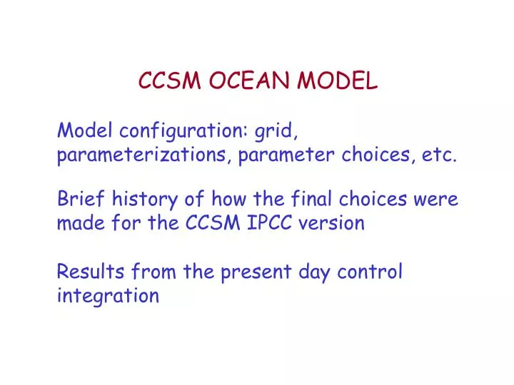
CCSM OCEAN MODEL. Model configuration: grid, parameterizations, parameter choices, etc. Brief history of how the final choices were made for the CCSM IPCC version. Results from the present day control integration. CCSM OCEAN MODEL. Based on the Parallel Ocean Program (POP 1.4) from LANL.

E N D
CCSM OCEAN MODEL Model configuration: grid, parameterizations, parameter choices, etc. Brief history of how the final choices were made for the CCSM IPCC version Results from the present day control integration
CCSM OCEAN MODEL Based on the Parallel Ocean Program (POP 1.4) from LANL GRID: - x1 displaced pole grid w/ 320x384 grid points - The pole is displaced into Greenland at 80oN, 40oW - The zonal resolution is constant at 1.125o - The meridional resolution varies: * 0.27o at Eq., 0.54 at 33oS * in the NH, the min and max resolutions are 0.38o and 0.65o away from the tropics - There are 40 levels in the vertical, monotonically increasing from 10 m near the surface to 250 m in the deep ocean. The min and max depths are 30 m and 5500 m.
The initial conditions are Levitus/PHC2 January-mean T and S and state of rest. • Ideal age is included as a tracer. • The tracers are advected using a third-order upwinding scheme. • A new version of the EOS from McDougall et al. (2003) is used. • The surface layer is variable, but we use virtual salt fluxes. Therefore, the global ocean volume is constant. • The time step is 1 hr. • The monthly-mean output files are in netCDF.
LATERAL TRACER MIXING • Gent-McWilliams (1990) isopycnal transport parameterization • Skew-flux (skewtion) form of Griffies(1998) • Both isopycnal and thickness diffusion coefficients are constant at 600 m2 s-1 • Both tapered when the isopycnal slopes get steep (starting at slope=0.18 w/ max slope=0.3) • Additional tapering within the boundary layer if the slopes are too steep • No background (horizontal) diffusion is used
HORIZONTAL MOMENTUM DIFFUSION • Horizontal viscosity is an anisotropic Laplacian operator following Smith and McWilliams (2003) formulation • East-west and north-south are the anisotropic directions • Both coefficients are spatially and temporally variable and depend on the local deformation rate following Smagorinsky (1963) CA = CB = 8 A1 = max[GRID REYNOLDS NUMBER(lat,depth), 1000] m2 s-1 B1 = max[MUNK VISCOUS LAYER(lon,lat,depth), 1000] m2 s-1
VERTICAL MIXING SCHEME • KPP scheme of Large et al. (1994) • - The current implementation is slightly different than the earlier versions Background diffusion = 0.1 (surface) – 1.0 (bottom) cm2 s-1 (mid-value occurs at 1000 m) PrT = 10. Double diffusion is on
SHORT-WAVE HEAT FLUX • The short-wave absorption is based on the chlorophyll amount • The climatological monthly-mean chlorophyll distributions from Ohlmann (2003) are used • The ocean model is coupled once a day, BUT a diurnal cycle is implemented for the short-wave heat flux
ROAD TO THE FINAL-ONE A low no no no no B high no no no yes C high yes no no yes D high yes yes yes yes E high yes yes yes no Ice albedo Tuned cloud forcing Longer atm tuning Best land IC Ocn s-w diurnal cycle Atm resolution is T85 T42 equivalents are denoted by primes (e.g. D’)
SENSITIVITY TO DIURNAL CYCLE WITH D E WITHOUT
NCEP WITH (D) WITHOUT (E)
STATUS OF (PUBLIC) INTEGRATIONS EXPERIMENT CASE YEAR T42-x1 control T85-x1 control T85-x1 1870 T85-x1 1% CO2/yr 2x2.5-x1 FV control b30.004 b30.009 b30.013 b30.014 b30.015 371 211 197 ?? 23