Download
1 / 30
300 likes | 326 Views
Model of solar faculae А.А. Solov’ev , solov@gaoran.ru. Pulkovo observatory 2018. Three classes of magnetic features in the plages of active regions.

E N D
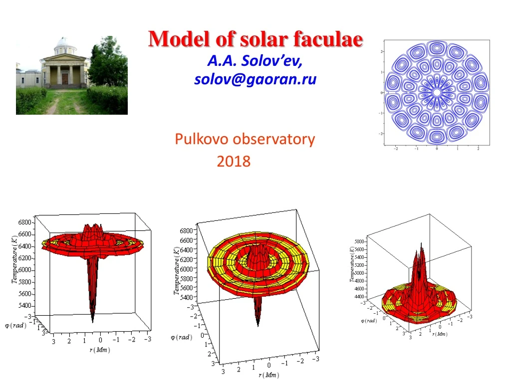
Model of solar faculae А.А. Solov’ev,solov@gaoran.ru Pulkovo observatory 2018
Three classes of magnetic features in the plages of active regions • As it known “There appear to be three distinct classes of magnetic features in the plage—small flux tubes, knots, and pores… There appears to be a nearly continuous interchange between these three states. Magnetogram movies show that on a spatial scale of a half-arcsecond and a temporal scale of minutes the small-scale magnetic field structures—flux tubes—are in constant motion”. • (A. M. Title et al, ApJ (1992) 393,782-794)
FIRST CLASS OF STUCTURES • A lot of work has been devoted to the study of structures of the first class (B.de Ponteieu et al. Ap.J 646,1405-1420,2006; T.E.Berger et al. New Solar Physics with Solar-B mission ASP Conf. Series 2007 369,103-112;) and many others. These ephemeral moving magnetic structures have granular scales (0.5-1 arcseconds and life-time 5-10 minutes) • Their physical nature can be well described numerically in the terms of magnetoconvection (Keller C.U et al ApJ. 607, L59-L62, 2004)
Second class of magnetic structures observed in plages of active regions • Solar facular knots are relatively stable and long-lived (up to 1 day or more) bright active formations with a diameter 3-8 Mm and fine (about 1 Mm or less) magnetic structure with magnetic field strengths from 250 G to 1000 G • Just these objects are regarded here. • The stationary MHD problem is solved and analytical formulae are derived for calculation the pressure, density, temperature, and Alfven Mach number in the configuration from the corresponding magnetic field structure. • The facular knot is introduced in a hydrostatic atmosphere defined by the model Avrett &Loeser (2008) and is surrounded by a weak (2G) external field corresponding to the global magnetic field on the solar surface (A.M.Title, C.J.Schrijver, ASP Conf. Series. 1998, Vol.154, 345-358)
Temperature • The calculated temperature profiles of the facular knot at the level of the photosphere have a specific shape: the temperature on the facular axis is lower than that in the surroundings but in the nearest vicinities of the axis and at the periphery of the knot, the gas is 200-100 K hotter than the surroundings. • Here, on the level of photosphere, the model describes both the central darkening of the faculae (like Wilson depression in sunspots) and also ring, semi-ring and segmental facular brightenings observed with New Swedish 1-m Telescope at high angular resolution (Lites et al.2004). • In the temperature minimum region (z = 525 km), the central dip in T-profile disappears and the facula as a whole is hotter than the chromosphere.
Temperature • At all heights of the chromosphere the temperature of the faculae is higher than surrounding environment at the same level. • This difference is particularly significant at heights of 1.5 and 2.2 Mm, where the main contribution to gas pressure within the facular node makes a pressure of the external magnetic field, which at these heights is already comparable with the internal magnetic field of the facula and even begins to surpass it. . • Apparently, just at these layers the facular magnetic flux tube forms the bright phenomena which are designated by observers as flocculi.
Equations of stationary MHD • The energy transport equation which has a very complicated form for solar plasma is left undetermined.
Derivation of the governing equation • According to stationary ideal MHD, the plasma flow takes place along the magnetic field lines: • Here Alfven Mach number is the ratio of the plasma fluid velocity and the corresponding Alfven velocity. It follows: • the factor is not change along the magnetic field line but can vary arbitrarily as we move to an another field line. • After a number of transformations we get the basic Equation of the problem For every given magnetic configuration B we can calculate all the required physical parameters of the system.
Magnetic structure of stationary facular node • Let the magnetic field has the form: • Pressure balance in azimuthal direction
General magnetic structure • Flow function: • is an arbitrary function!!
. Angular dependence, Alfven Mach number The R.H.S. of this expression doesn’t contain the angular dependence : Consequently, we must take: Now, the L.H.S. of the Eq. for the density doesn’t depend on the angle, consequently this dependence disappears for the distribution of plasma density which in our configuration happens to have an axially symmetric form:
Equations for pressure and density • Finally we have:
Magnetic field of faculae knot • As a base, we take Schazman (1965) solution, • Bo is the magnetic field strength at the level of z = z0 , is the reciprocalheight scale. • We introduce some correction in the solution
The function Z(z) in the form of distorted step with zo=0.125 Mm For z = 0, at the photosphere level, Z(0) =0.622
working formulas • Using the corrected expressions we have
Photospheric level, z = 0. Temperature of plasma is 6583K • B0=1000G
Photosphere • Bo = 500G Bo = 250G
Z =525 km, temperature min • B0= 1000G Bo =500 G
Level of z = 1032км, the temperature of chromosphere is 6315К • B0=1000G B0=500G
. Level with z = 1520km, the temperature of chromosphere is 6623К • Bo = 1000G Bo =500G • Bo =500G
Level near the transition region, z =2083km, the temperature of the chromosphere is 7729 K. • Bo =1000G Bo =500G
Conclusions • A steady MHD model for the solar facular knot with fine filamentary structure of the magnetic field is constructed. • Analytical formulae for the calculation of gas pressure, density, Alfven Mach number and temperature according to the given magnetic configuration are derived. • Facular magnetic configuration with external magnetic field of 2G is introduced for the solar atmosphere which is described by the modern empirical model Avrett & Loeser (2008).
3. Numerically evaluated profiles of plasma temperature inside the facular knot at the level of the photosphere have a specific form: there is negative contrast at the axis (Wilson’s depression), but at the nearest vicinities the temperature sharply rises and local rise in temperature of the individual facular granules above the surrounding medium is observed all along the area of the facular knot. • The geometry of profiles doesn’t change even for large magnetic field variations. The variation of magnetic field only results in the change of the temperature range in the facular knot.
At the height of the temperature minimum (525 км), the central temperature dip disappears and the entire profile of the faculae is located above the background and has temperature one and a half times more that of the ambient plasma at this level. 5. At the heights of 1500-2000 km above the photosphere, the gas of faculae is two and half times hotter than the ambient plasma at the same level. 6. Most likely that due to the fact that faculae have a high temperature at the heights above 1 Mm, the observers distinguish between faculae and flocculi as two different phenomena. Faculae are considered to be photospheric and lower chromospheric phenomena and flocculi or plages are considered to be the upper chromospheric phenomena.
7. In whole, the parameters and results of calculations of the model are in good correspondence with the most recent observational data of the solar faculae. This model, in particular, describes at the first time periodic concentric rings, half rings and segmental brightening observed in the facular fields at high angular resolution at the level of photosphere (Lites et al., 2004; Berger et al., 2007). The work was supported by the Russian Foundation of Basic Researches (project № 18-02-00168).
Model of twisted flux tube on the base of E.Schatzman force-free solution (IAU Symp. 22,337.1965)


![MBN Explorer [ 1,2] is a multi-purpose software package designed to study molecular systems of](https://cdn1.slideserve.com/2099881/slide1-dt.jpg)