Download
1 / 42
420 likes | 568 Views
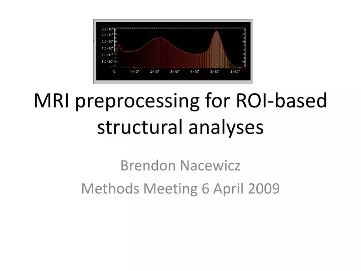
MRI preprocessing for ROI-based structural analyses. Brendon Nacewicz Methods Meeting 6 April 2009. Goals. Motivations/considerations for anatomical preprocessing T1 histogram Partial voluming: solved by rigorous numerical criteria (or oversampling) Convey what has worked well

E N D
MRI preprocessing for ROI-based structural analyses Brendon Nacewicz Methods Meeting 6 April 2009
Goals • Motivations/considerations for anatomical preprocessing • T1 histogram • Partial voluming: solved by rigorous numerical criteria (or oversampling) • Convey what has worked well • better than fancy programs with high-order parametric fits in one case • Convey what hasn’t worked: • Don’t reinvent the wheel • Segmentation of thalamic tissue from internal & external capsule • Non-interactive skull stripping is not good enough for VBM-type analyses of cortex
Disclaimer: Define kludge: A kludge (or kluge) is a workaround, an ad hoc engineering solution, a clumsy or inelegant solution to a problem, typically using parts that are cobbled together. • Probably none of my scripts is the fastest most computationally efficient implementation This is deliberate because: • I’m all about open source • That means AFNI, FSL, Python (formerly PERL) • No MATLAB, IDL or their emulators (Octave, etc) • All standard distributions (no numpy, etc) • Modularized but not truly object oriented • Tried to emulate pedagogical value of Tom’s afnigui: • You see the final command for every step • I think everyone should have a mac laptop and should be able to run my scripts on them
Another disclaimer: • I’m an end-user: • I don’t care about K-means vs SVD vs XKCD segmentation... • I don’t care how the code works • I care only what gives the most anatomically consistent results
Outline • Superestore() – formerly semi-interactive preprocessing script • Degrader() – a triumph of Oakes-assisted practicality • Contraster() – reducing inter-rater variability since 2008 • Superseg() – Separating GM from CSF for spectroscopy voxel tissue content Example of how this all helped
Motivation • Amygdala tracing is very difficult • Need to train up eyes for visual discrimination • Visual discrimination is *very low-level brain process* Implications • Visual Quadrant specific • Center the window in your visual field • Flip images to work on other hemisphere • Image Orientation specific (pathological plane) • Contrast sensitive Goal: every time you look at a voxel of a brain image, that screen pixel is exactly the same gray for the same tissue type
This is the goal: Good separation of peaks GM WM CSF Minimally Skewed Distributions
OK, this is what you really have (quad coil) • But whether you know it or not, you’re using the 8-channel coil from now on...
Original Contrasted (automatic contrasting) Histograms from skull-on images require log scale due to huge peaks of non-zero noise outside skull at low intensities and excess skull & vessels at highest intensities
Original Contrasted Noskl (*histo no longer log) With the skull removed and the center of the white matter distribution aligned to 80% of range: GM & WM distributions are flat & have huge tails (sub-gaussian).
This is what we’ll end up with (8-channel) *not log scale
superestore.py(A slow-paced story about FAST) • Originally called IRrestore.pl • Inspired by this: • fast -A: • aligns brain to MNI152 template • then uses spatial priors to constrain segmentation • Use with –or option to output restored image • Awesome except: • Subtly different
New strategy (IRrestore.pl): • Align brain to MNI & bring MNI brain *with skull* to original image space • Do rough bias correction in mFAST • Get good skull strip using BET interactively by changing location coordinates for center of brain • Remove vessels for better alignment • Now do Fast –A with great skull stripping
This is what came out(and it was great at the time) New Problem • For tracing: need to see outside of brain to identify vessel artifact • Used –ob to “output bias” • Can then apply bias map back to original brain image and everything’s perfect! Almost.
You need to know this if you plan to use FSL’s mFAST! • mFast –ob for T1 & T2 gives • T1_bias • T2_bias • The way it works is this: • T1_bias removes ½ from T1 • T1_bias adds ½ to T2 • You must use: • T1xT1_bias/T2_bias • Note: you can’t do this in fslmaths • fslmaths T1 –div T1_bias = 0, since first argument tells it to use 16-bit and bias maps are float with values mostly 0-1
Whew! That’s better... • Same goes for using mfast with the MNI152 brain • Thus: • T1_superestore = T1*T1_bias/MNI_bias
This was really involved & time consuming • Took about 40 minutes per brain for whole cycle • Lots of intermediate files • AFNI saves the day: • New version of 3dSkullStrip • Stole FSL bias correction & did exactly what IRrestore.pl script did • I am not a unique snowflake Current recommendation: use 3dskullstrip with recommended parameters (defaults in superseg2.py or in superestore.py)
Goal: • Find center of bright spot • Terry says ~“Lots of groups are trying higher parameter segmentations and they don’t work. Constrain it to the simplest thing you can” • Too difficult to use arbitrary cost • If you can get rough WM mask, use distribution of WM
Strategy Calculate center of bright spot using 3dcalc’s handy i,j,k bricks e.g. (mask*i) = gives i coordinates for averaging Make binary mask of 97-98th percentile of white matter intensities Weight gradient by some scalar & remove from image using some cost function Create simple linear gradient intensity = max(image_dims)-1*distance_from_center Iamge_dims & distance in pixels
Why not 99th %ile? • Estimated center of bright spot using 99th %ile always seemed a little bit inferior/ventral • Answer: Vessels (+vessel artifact*optic chiasm)
You can use a gray matter mask, but you don’t have to • Center from WM 97th-98th %ile compared to GM 99th %ile • Center of brightspot differed by less than 3mm in all directions (often identical) • No need to use GM mask • You can if you’re obsessive though...
Gradient: linear gradient ranging from max(i,j,k brik dimensions) at center to max-1*distance_in_voxels(use max brik dimensions so that it’s never < 0) • command = "3dcalc -a "+orig+(".hdr"*(isafni-1))+" -prefix "+gradient+" -expr '("+radius+"**2-(k-"+k+")**2)/"+radius+"**2*("+radius+"**2-(j-"+j+")**2)/"+radius+"**2*("+radius+"**2-(i-"+i+")**2)/"+radius+"**2' 2>/dev/null” • This makes a gradient that decreases w/slope -1 with distance (in voxels) from center of bright spot and maximum of 128 if the largest dimension is 256
Actual application & cost: • Actual application does this: • Image+(1-gradient)*image*strength • Note: instead of subtracting the gradient, it adds mathematical inverse of gradient*image to keep values > 0 • How to pick strength? • Original reasoning: if same number of voxels is getting more uniformly distributed, peak of histogram (mode) should increase • Fail! • Adding some multiple of image*(1-gradient) eventually amounts to image^multiple for some regions • This means the entire distribution is spread upward in intensity • Added correction factor to prevent this but still very difficult to contain • Final solution: • Used the following correction factor • (image+(1-gradient)*image*strength)/ max(1,(image_mean_intensity+gradient_mean_intensity*strength)/image_mean_intensity) • COST: calculate actual skew (3rd moment) and find zero-crossing
This works on every brain in /study/outlier_data/structural* • It works even if there’s no tissue at the center of the gradient
This works on every brain in /study/outlier_data/structural* *Although it can’t create contrast where the original image had too little
contraster.py • get_histo_info() • Takes a mask file • Basically will load 3dhistog info into 2 arrays with a default of 250 bins (3dhistog defaults to 100) • Returns 2 arrays (lists) • maxindex() • Give it an array, it finds the max & returns: • (max, maxindex) • contraster() • Takes a brain (& a mask) and rescales so peak of histogram (mode) is at 80% of 16-bit range (.8*2^16) • Give it a white matter mask
Contraster.py • Forces image to use short/16-bit • (let’s see you do that in FSL) • Assumes valuable information in image is 2500 or below (this is typical) • Images can store intensities up to 2^16 = 65536 • Peak of white matter histogram = mode • Move this to 80% of dynamic range (65536)
Disco Ball Brain: • Interested in a 2swap? • Once in a while, this & other scripts will produce a result that needs byte swapping. This is easily fixed (in seconds) by running afni’s 2swap command on the .BRIK file
superseg2.py • I have tried countless tests of iterative bias correction & segmentation • I have varied the order of operations several different ways • This is what works the best for the most datasets! • In other words, this is almost purely empirical (not analytical)
Original Quad Coil Image Superseg2.py • I tried all sorts of things to get a better gray matter-CSF distinction in the area of the amygdala • In the end, I needed a way to push the distributions of the different tissue types further apart • How to solve this? T1_degrad_superestore_contrasted T1_degrad_superseg_contrasted T1_degrad_superestore_contrasted Too Much Overlap! Too Much Awesome!
Superseg2.py 8-channel image after degrader & superseg • Works great on 8-channel too! • I use as: • Run superseg 1X to get WM mask • Run degrader with original image & WM mask as inputs • Rerun superseg on T1_degrad+orig • Viola! • Cons: • Squaring the image squares the noise in a way that true averaging wouldn’t • If you run it in original space (unsmoothed), then AC-PC align or rotate to “pathological plane”, this will get smoothed out • Could also use 3danisosmooth • I have a wrapper for that which describes some of the best parameters I’ve found
Superseg2.py FAQ • Can I just square my brain images to improve contrast? • No. The only reason we can do this is because we have an excellent removal of the gradient. You square the gradient, and you’ll get a ridiculous result. Also, I know my peaks are going to be well contained because I put them exactly where I want them (white matter is centered at 80%). If you square images randomly, you don’t know where your peaks start or will end up. • Why 16-bit? • 8-bit (256 grays) is easiest for numerical criteria for tracing • But, I keep the images at 16-bit precision for partial-volume stuff from all the rotations • Solution: Once you rotate it to the pathological plane • Change it to 8-bit without calibration factor in spam • Alternatively (I never got it to work): • maybe use 3dcalc to apply a scaling (maybe 256/65536) and then convert to 8-bit • Should I run superseg on AC-PC aligned brains? • No. It will work just fine, but my scripts are designed to be run in original space so you can then apply your own tlrc or acpc alignment • If you use it on one of these more-processed images, it’s very difficult to go backwards (e.g. AC-PC to original space) like if you wanted to mask a DTI image in native space • I have a script that might help take ROIs back to original space though if you traced in ac-pc space... • Where do the scripts live? • They are on /study/amygdala/preprocessing/python_scripts • Most of the code is in brImaging.py and the respective scripts • I have (simplistic) wrappers for each of the scripts, which could be added to your path and run as executables* • *You may have to change the path to python on the first line: E.g. #! /usr/bin/python works fine for standard python install #! /apps/scientific_45/bin/bin_dist/python used to work at waisman
What does this buy us? Good separation of peaks GM WM CSF Minimally Skewed Distributions
Lateral amygdala nucleus autdti116
More validation of Lateral Amygdala Nucleus(Gold standard: average of 4 Jamie brains) Inverted Weigert Stain (Unlocked Mai Atlas PDF)
Allows new tracing criterion • Q: Is it amygdala or partial volume hippocampus (alveus)? • Is it darker than rest of amygdala? • If no: it’s hippocampus • If yes: it’s amygdala
Other Scripts for ROIs • Midway() – Using linear algebra to most equitably distort your multiple acquisitions • Blind() – When you have no friends, you have to blind your own data • fractionalize.pl – Takes your ROIs that you rotated back to AC-PC space all the way back to original space using absolute volume to pick threshold for partial volume effects (iterative)