Download
1 / 55
550 likes | 702 Views
High-Precision Astrometry of the S5 polarcap sources. Jose C. Guirado (Univ. Valencia) & J.M. Marcaide (UV), I. Martí-Vidal (MPIfR), S. Jiménez (UV), E. Ros (UV). The S5 Polar Cap Sample. Studied in MPIfR since 80s (Eckart et al., 1987, Witzel et al., 1988, etc.)

E N D
High-Precision Astrometry of the S5 polarcap sources Jose C. Guirado (Univ. Valencia) & J.M. Marcaide (UV), I. Martí-Vidal (MPIfR), S. Jiménez (UV), E. Ros (UV)
The S5 Polar Cap Sample • Studied in MPIfR since 80s (Eckart et al., 1987, Witzel et al., 1988, etc.) • Flat spectrum Radiosources: • 8 QSOs • 5 BL-Lac objects
GLOBAL HIGH-PRECISION ASTROMETRY Epoch 1 Epoch 2 We can study astrometric variations in time and/or frequency
GLOBAL HIGH-PRECISION ASTROMETRY astrometric variations in time and/orfrequency
GLOBAL HIGH-PRECISION ASTROMETRY astrometric variations in time and/orfrequency
GLOBAL HIGH-PRECISION ASTROMETRY astrometric variations in time and/orfrequency
GLOBAL HIGH-PRECISION ASTROMETRY astrometric variations in time and/orfrequency
VLBA OBSERVATIONS Epoch Frequency (GHz) 8.4 15.4 43 1997.93 1999.41 1999.57 2000.46 2001.04 2001.09 2001.71 2004.53 2004.62 2005.45
PHASE-DELAY ASTROMETRY • Relative separation determination by means of least squares fits: • Homogeneous sampling of all sources at different frequencies.
geo(t)+ ion(,E(t))+ (t)= trop(E(t))+ 30 ms 5-9 ns (E=90º) 0.1-3 ns (E=90º) + str(,t)+ instrum(t) 0-300 ps 1 ps/s The Fitting Model
geo(t)+ ion(,E(t))+ (t)= trop(E(t))+ 30 ms 5-9 ns (E=90º) 0.1-3 ns (E=90º) + str(,t)+ instrum(t) 0-300 ps 1 ps/s The Fitting Model TECTONICS, TIDES, AND RELATIVISTIC MODELS
geo(t)+ ion(,E(t))+ (t)= trop(E(t))+ 30 ms 5-9 ns (E=90º) 0.1-3 ns (E=90º) + str(,t)+ instrum(t) 0-300 ps 1 ps/s The Fitting Model TECTONICS, TIDES, AND RELATIVISTIC MODELS METEOROLOGY MEASUREMENTS
geo(t)+ ion(,E(t))+ (t)= trop(E(t))+ 30 ms 5-9 ns (E=90º) 0.1-3 ns (E=90º) + str(,t)+ instrum(t) 0-300 ps 1 ps/s The Fitting Model TECTONICS, TIDES, AND RELATIVISTIC MODELS GPS (IONEX TABLES) METEOROLOGY MEASUREMENTS
geo(t)+ ion(,E(t))+ (t)= trop(E(t))+ 30 ms 5-9 ns (E=90º) 0.1-3 ns (E=90º) + str(,t)+ instrum(t) 0-300 ps 1 ps/s The Fitting Model TECTONICS, TIDES, AND RELATIVISTIC MODELS GPS (IONEX TABLES) METEOROLOGY MEASUREMENTS MAPS OF RADIOSOURCES
geo(t)+ ion(,E(t))+ (t)= trop(E(t))+ 30 ms 5-9 ns (E=90º) 0.1-3 ns (E=90º) + str(,t)+ instrum(t) 0-300 ps 1 ps/s The Fitting Model TECTONICS, TIDES, AND RELATIVISTIC MODELS GPS (IONEX TABLES) METEOROLOGY MEASUREMENTS MAPS OF RADIOSOURCES WLSF ESTIMATE
geo(t)+ ion(,E(t))+ (t)= trop(E(t))+ 30 ms 5-9 ns (E=90º) 0.1-3 ns (E=90º) + str(,t)+ instrum(t) 0-300 ps 1 ps/s The Fitting Model TECTONICS, TIDES, AND RELATIVISTIC MODELS GPS (IONEX TABLES) METEOROLOGY MEASUREMENTS MAPS OF RADIOSOURCES WLSF ESTIMATE The Fitting Software • Geometric model and fitting procedures computed with the University of Valencia Precision Astrometry Package (UVPAP): • - Possibility of multisource differential astrometry
The Fitting Strategy • Find a preliminary model by fitting the clock drifts and the atmospheric zenith delays to the GROUP DELAY data. • Use the resulting model to estimate the phase ambiguities of the PHASE DELAY (pre-connection). • Refine the phase connection and perform the astrometric analysis (check the quality of the differential observables).
EPOCH 2000.46, 15GHz PHASE-CONNECTION -Time between obs. ~ 120 s -2 cycle at 15 GHz ~ 65 ps THUS, -Residual rates should be lower than 33ps/120ps ~0.3 ps/s
Check Phase Closures Phase closures should be NULL for point-like sources, or for observables from which we extract all the source structure information.
Check Phase Closures Phase closures should be NULL for point-like sources, or for observables from which we extract all the source structure information.
Automatic Phase Connector The Algorithm: - For a given scan: • Finds which baseline appears more times in the set of non-zero closures. • Adds and subtracts 1 phase cycle to the delay of that baseline. Computes the score corresponding to each of these corrections: • score = (# of closures moved closer to 0) – (# of closures moved away from zero). • The highest score will determine which correction is applieddefinitely. • Recomputes the closures and repeats the previous steps until all closures are zero. Applies the set of corrections found for the actual scan to the next scan, before it computes the closures of that new scan.
Automatic Phase Connector Corrected baselines: Closures: (Simulations) Baselines:
Antenna-based corrections: Antenna: OV Source: 04 Nº of ambs: +1
When things are not as expected... Residual delay rate (ps/s) Baselines with SC Weather dependent...
Relative Position Uncertainty Triangles = RA uncertainties Squares = Dec uncertainties
Results: differential positions • We find some large corrections of the relative sources coordinates with respect to the ICRF positions. Nevertheless, our astrometric results are not directly comparable to the ICRF: • -Our astrometric corrections are defined with respect to the “phase centers” of the maps. Our astrometry considers, then, the structures of the sources. • -Source opacity effects could be present while comparing the source positions observed at 15GHz and 8.4/2.3 GHz • Mean corrections are: • 278as in RA • 170as in DEC
Some Results Astrometry of 0212+735 15 GHz
Some Results Astrometry of 0212+735 15 GHz 43 GHz
Some Results Astrometry of 1928+738
Some Results Astrometry of 1928+738 Ros et al. 2000
Some Results Astrometry of 1928+738 Ros et al. 2000
Results:1928+738 time series 43 GHz 15.4 GHz 8.4 GHz Q1999.01 X1988.83 K1999.57 X1991.89 K2000.46 X2001.09 C1985.8 Q2004.62 X2004.53
Results:1928+738 time series 43 GHz 15.4 GHz 8.4 GHz Q1999.01 X1988.83 K1999.57 X1991.89 K2000.46 X2001.09 C1985.8 Q2004.62 X2004.53
Results:1928+738 time series 43 GHz 15.4 GHz 8.4 GHz Q1999.01 X1988.83 K1999.57 X1991.89 K2000.46 X2001.09 C1985.8 Q2004.62 X2004.53