Download
1 / 38
380 likes | 488 Views
Intelligent Systems (AI-2) Computer Science cpsc422 , Lecture 14 Feb, 5, 2014. Slide credit: some slides adapted from Stuart Russell (Berkeley). R&R systems BIG PICTURE. Stochastic. Deterministic. Environment. Problem. Arc Consistency. Search. Constraint Satisfaction. Vars +

E N D
Intelligent Systems (AI-2) Computer Science cpsc422, Lecture 14 Feb, 5, 2014 Slide credit: some slides adapted from Stuart Russell (Berkeley) CPSC 422, Lecture 14
R&R systems BIG PICTURE Stochastic Deterministic Environment Problem Arc Consistency Search Constraint Satisfaction Vars + Constraints SLS Static Belief Nets Var. Elimination Logics Query Approx. Inference Search Markov Chains and HMMs Temporal. Inference Sequential Decision Nets STRIPS Var. Elimination Markov Decision Processes Planning Value Iteration Search Representation POMDPs Approx. Inference Reasoning Technique CPSC 502, Lecture 13
Lecture Overview(Temporal Inference) • Filtering (posterior distribution over the current state given evidence to date) • From intuitive explanation to formal derivation • Example • Prediction (posterior distribution over a future state given evidence to date) • (start) Smoothing (posterior distribution over a past state given all evidence to date) CPSC 422, Lecture 14
Markov Models Markov Chains Hidden Markov Model Partially Observable Markov Decision Processes (POMDPs) Markov Decision Processes (MDPs) CPSC422, Lecture 5
Hidden Markov Model • A Hidden Markov Model (HMM) starts with a Markov chain, and adds a noisy observation/evidence about the state at each time step: • |domain(X)| = k • |domain(E)| = h • P (X0) specifies initial conditions • P (Xt+1|Xt) specifies the dynamics • P (Et |St) specifies the sensor model CPSC422, Lecture 5
Simple Example (We’ll use this as a running example) • Guard stuck in a high-security bunker • Would like to know if it is raining outside • Can only tell by looking at whether his boss comes into the bunker with an umbrella every day Transition model State variables Observation model Observable variables
Useful inference in HMMs • In general (Filtering): compute the posterior distribution over the current state given all evidence to date P(Xt| e0:t) CPSC422, Lecture 5
Intuitive Explanation for filtering recursive formula P(Xt| e0:t) CPSC422, Lecture 5
Filtering • Idea: recursive approach • Compute filtering up to time t-1, and then include the evidence for time t (recursive estimation) • P(Xt|e0:t) = P(Xt |e0:t-1,et) dividing up the evidence = αP(et| Xt, e0:t-1) P(Xt| e0:t-1) WHY? = αP(et| Xt) P(Xt | e0:t-1) WHY? • A. Bayes Rule • B. Cond. Independence • C. Product Rule One step prediction of current state given evidence up to t-1 Inclusion of new evidence: this is available from.. • So we only need to compute P(Xt | e0:t-1)
why? Filtering Prove it? • Compute P(Xt | e0:t-1) • P(Xt | e0:t-1) = ∑xt-1P(Xt, xt-1 |e0:t-1) = ∑xt-1P(Xt | xt-1 , e0:t-1) P(xt-1 | e0:t-1) = • = ∑xt-1P(Xt | xt-1 ) P(xt-1 | e0:t-1) because of.. Filtering at time t-1 Transition model! • Putting it all together, we have the desired recursive formulation • P(Xt |e0:t) = αP(et| Xt) ∑xt-1P(Xt | xt-1 ) P(xt-1 | e0:t-1) Filtering at time t-1 Inclusion of new evidence (sensor model) Propagation to time t • P(Xt-1 | e0:t-1) can be seen as a message f0:t-1 that is propagated forward along the sequence, modified by each transition and updated by each observation
Filtering • Thus, the recursive definition of filtering at time t in terms of filtering at time t-1 can be expressed as a FORWARD procedure • f0:t =α FORWARD (f0:t-1, et) • which implements the update described in P(Xt |e0:t) = αP(et| Xt) ∑xt-1P(Xt | xt-1 ) P(xt-1 | e0:t-1) Filtering at time t-1 Inclusion of new evidence (sensor model) Propagation to time t
Analysis of Filtering • Because of the recursive definition in terms for the forward message, when all variables are discrete the time for each update is constant (i.e. independent of t ) • The constant depends of course on the size of the state space and the type of temporal model
Rain Example • Suppose our security guard came with a prior belief of 0.5 that it rained on day 0, just before the observation sequence started. • Without loss of generality, this can be modeled with a fictitious state R0 with no associated observation and P(R0) = <0.5, 0.5> • Day 1: umbrella appears (u1). Thus • P(R1 | e0:t-1) = P(R1) = ∑r0P(R1 | r0 ) P(r0) • = <0.7, 0.3> * 0.5 + <0.3,0.7> * 0.5 = <0.5,0.5> 0.5 0.5 TRUE 0.5 FALSE 0.5 Rain2 Rain0 Rain1 Umbrella2 Umbrella1
Rain Example • Updating this with evidence from for t =1 (umbrella appeared) gives • P(R1| u1) = αP(u1| R1) P(R1) = • α<0.9, 0.2><0.5,0.5> = α<0.45, 0.1> ~ <0.818, 0.182> • Day 2: umbella appears (u2). Thus • P(R2 | e0:t-1) = P(R2 | u1) = ∑r1P(R2 | r1 ) P(r1| u1) = • = <0.7, 0.3> * 0.818 + <0.3,0.7> * 0.182 ~ <0.627,0.373> 0.627 0.373 0.5 0.5 TRUE 0.5 FALSE 0.5 0.818 0.182 Rain2 Rain0 Rain1 Umbrella2 Umbrella1
Rain Example • Updating this with evidence from for t =2 (umbrella appeared) gives • P(R2| u1 , u2) = αP(u2| R2) P(R2| u1) = • α<0.9, 0.2><0.627,0.373> = α<0.565, 0.075> ~ <0.883, 0.117> • Intuitively, the probability of rain increases, because the umbrella appears twice in a row 0.627 0.373 0.5 0.5 TRUE 0.5 FALSE 0.5 0.883 0.117 0.818 0.182 Rain2 Rain0 Rain1 Umbrella2 Umbrella1
Practice exercise (home) • Compute filtering at t3 if the 3rd observation/evidence is no umbrella CPSC 422, Lecture 14
Lecture Overview • Filtering (posterior distribution over the current state given evidence to date) • From intuitive explanation to formal derivation • Example • Prediction (posterior distribution over a future state given evidence to date) • (start) Smoothing (posterior distribution over a past state given all evidence to date) CPSC 422, Lecture 14
Prediction (P(Xt+k+1 | e0:t)) • Can be seen as filtering without addition of new evidence • In fact, filtering already contains a one-step prediction • P(Xt |e0:t) = αP(et| Xt) ∑xt-1P(Xt | xt-1 ) P(xt-1 | e0:t-1) Filtering at time t-1 Inclusion of new evidence (sensor model) Propagation to time t • We need to show how to recursively predict the state at time t+k +1 from a prediction for state t + k • P(Xt+k+1 | e0:t) = ∑xt+kP(Xt+k+1, xt+k|e0:t) = ∑xt+kP(Xt+k+1 | xt+k, e0:t) P(xt+k| e0:t) = • = ∑xt+kP(Xt+k+1 | xt+k) P(xt+k| e0:t) • Let‘s continue with the rain example and compute the probability of Rain on day four after having seen the umbrella in day one and two: P(R4| u1 , u2) Prediction for state t+ k Transition model
Rain Example • Prediction from day 2 to day 3 • P(X3 | e1:2) = ∑x2P(X3 | x2 ) P(x2 | e1:2) = ∑r2P(R3 | r2 ) P(r2 | u1 u2) = • = <0.7,0.3>*0.883 + <0.3,0.7>*0.117 = <0.618,0.265> + <0.035, 0.082> • = <0.653, 0.347> • Prediction from day 3 to day 4 • P(X4 | e1:2) = ∑x3P(X4 | x3 ) P(x3 | e1:2) = ∑r3P(R4 | r3 ) P(r3 | u1 u2) = • = <0.7,0.3>*0.653 + <0.3,0.7>*0.347= <0.457,0.196> + <0.104, 0.243> • = <0.561, 0.439> 0.627 0.373 0.5 0.5 0.561 0.439 0.653 0.347 0.5 0.5 0.883 0.117 0.818 0.182 Rain3 Rain3 Rain0 Rain1 Rain2 Umbrella3 Umbrella1 Umbrella2 Umbrella3
Rain Example • What happens if I try to predict further and further into the future? • A. Probability of Rain will oscillate • B. Probability of Rain will decrease indefinitely to zero • C. Probability of Rain will converge to a specific value
Rain Example • Intuitively, the probability that it will rain decreases for each successive day, as the influence of the observations from the first two days decays • What happens if I try to predict further and further into the future? • It can be shown that the predicted distribution converges to the stationary distribution of the Markov process defined by the transition model (<0.5,0.5> for the rain example) • When the convergence happens, I have basically lost all the information provided by the existing observations, and I can’t generate any meaningful prediction on states from this point on • The time necessary to reach this point is called mixing time. • The more uncertainty there is in the transition model, the shorter the mixing time will be • Basically, the more uncertainty there is in what happens at t+1 given that I know what happens in t, the faster the information that I gain from evidence on the state at t dissipates with time
Lecture Overview • Filtering (posterior distribution over the current state given evidence to date) • From intuitive explanation to formal derivation • Example • Prediction (posterior distribution over a future state given evidence to date) • (start) Smoothing (posterior distribution over a past state given all evidence to date) CPSC 422, Lecture 14
Smoothing • Smoothing: Compute the posterior distribution over a past state given all evidence to date • P(Xk |e0:t)for 1 ≤ k < t E0
Smoothing • P(Xk |e0:t) = P(Xk |e0:k,ek+1:t) dividing up the evidence = αP(Xk| e0:k) P(ek+1:t| Xk, e0:k) using… = αP(Xk| e0:k) P(ek+1:t| Xk) using… forward message from filtering up to state k, f 0:k backward message, b k+1:t computed by a recursive process that runs backwards from t
Smoothing • P(Xk |e0:t) = P(Xk |e0:k,ek+1:t) dividing up the evidence = αP(Xk| e0:k) P(ek+1:t| Xk, e0:k) using Bayes Rule = αP(Xk| e0:k) P(ek+1:t| Xk) By Markov assumption on evidence forward message from filtering up to state k, f 0:k backward message, b k+1:t computed by a recursive process that runs backwards from t
CPSC 422, Lecture 14 Learning Goals for today’s class • You can: • Describe Filtering and derive it by manipulating probabilities • Describe Prediction and derive it by manipulating probabilities • Describe Smoothing and derive it by manipulating probabilities
CPSC 422, Lecture 14 TODO for Fri • Complete and submit Assignment-1 • Assignment-2 will be posted on Fri • RL, Approx. Inference in BN, Temporal Models) – start working on it – • due Feb 19 (it may take longer that first one) • Reading Textbook Chp. 6.5 • DLS Talk tomorrow 3:30 on Natural Language Processing (applies Reinforcement Learning!)
Other useful HMM Inferences • Smoothing (posterior distribution over a past state given all evidence to date) • P(Xk |e0:t) for 1 ≤ k < t • Most Likely Sequence(given the evidence seen so far) • argmaxx0:tP(X0:t| e0:t) CPSC 502, Lecture 10
Discussion • Note that the first-order Markov assumption implies that the state variables contain all the information necessary to characterize the probability distribution over the next time slice • Sometime this assumption is only an approximation of reality • The student’s morale today may be influenced by her learning progress over the course of a few days (more likely to be upset if she has been repeatedly failing to learn) • Whether it rains or not today may depend on the weather on more days than just the previous one • Possible fixes • Increase the order of the Markov Chain (e.g., add Raint-2 as a parent of Raint) • Add state variables that can compensate for the missing temporal information Such as?
Rain Network • We could add Month to each time slice to include season statistics Montht Montht+1 Montht-1 Raint+1 Raint-1 Raint Umbrellat+1 Umbrellat-1 Umbrellat
Pressuret+1 Pressuret Pressuret-1 Humidityt+1 Humidityt Humidityt-1 Temperaturet+1 Temperaturet Temperaturet-1 Raint-1 Raint Raint+1 Umbrellat-1 Umbrellat Umbrellat+1 Rain Network • Or we could add Temperature, Humidity and Pressure toinclude meteorological knowledge in the network
Rain Network • However, adding more state variables may require modelling their temporal dynamics in the network • Trick to get away with it • Add sensors that can tell me the value of each new variable at each specific point in time • The more reliable a sensor, the less important to include temporal dynamics to get accurate estimates of the corresponding variable Humidityt Humidityt-1 Pressuret-1 Pressuret Temperaturet-1 Temperaturet Raint Raint-1 Thermometert Thermometert-1 Barometert-1 Barometert Umbrellat Umbrellat-1
Overview • Modelling Evolving Worlds with DBNs • Simplifying Assumptions • Stationary Processes, Markov Assumption • Inference Tasks in Temporal Models • Filtering (posterior distribution over the current state given evidence to date) • Prediction (posterior distribution over a future state given evidence to date • Smoothing (posterior distribution over a past state given all evidence to date) • Most Likely Sequence (given the evidence seen so far) • Hidden Markov Models (HMM) • Application to Part-of-Speech Tagging • HMM and DBN
CPSC 502, Lecture 10 HMM: more agile terminology Formal Specification as five-tuple Set of States Output Alphabet Initial State Probabilities State Transition Probabilities Symbol Emission Probabilities
CPSC 502, Lecture 10 1. Initialization 2. Induction Complexity The forward procedure